28. AGX Model: PID Controller
This chapter describes the PID controller implementation in AGX Model.
In agxModel::PidController1D there is an implementation of a PID controller with the classic
gains for proportional, integral, and derivative gain described by the following mathematical expression:
where \(u\) is the out signal, also known as the Manipulated Variable (MV), and \(K_p\), \(K_i\), and \(K_d\) are the tuning parameters or proportional gain, integral gain, and derivative gain. In the figure below, Fig. 28.1, there is a schematic representation of the PID controller including the process the PID is controlling, known as the Plant.
The above equation is discretized with the forward Euler Method and this leads to an explicit solution of \(u(t)\). The error, \(e\), is calculated as the difference between the measured Process Variable (PV) on the Plant and the desired Set Point (SP), the derivative of the error is discretized as \(\frac{de}{dt} = \frac{e - e_{n-1}}{t - t_{n-1}}\), where \(e_{n-1}\) is the error from the previous time step and \(t - t_{n-1}\) is the time step. The integral part is approximated by adding up the error, \(e\), multiplied by the time step. This explicit solution of \(u(t)\) is relatively sensitive to high frequencies in the Plant.
The PID controller has an integral windup algorithm with both “clamping” and/or an integral back-calculation algorithm. The clamping is disabled per default and the back-calculation is activated if the PID controller are given constraints on the Manipulated Variable (MV). The backward calculation is done by recomputing the integral term to its previous state before the windup started and by that disabling the integration.

Fig. 28.1 Above is a schematic diagram over the PID controller. From left to right we have the error which is the difference between the Set Point (SP) and the Process Variable (PV). \(K\) represents the three gains and the block to the right represent the integral windup algorithm activated when the output signal, Manipulated Variable (MV), is outside the Plant input limits.
28.1. C++ example of PidController with ControllerHandler
It is possible to use the PID controller in a stand alone application but the agxModel::PidController1D is preferable to be used together with the agxModel::ControllerHandler which is a StepEventListener. The agxModel::ControllerHandler reads the Process Variable (PV) from the Plant, or controlled process, and lets the PID controller calculate a new Manipulated Variable (MV) with respect to the current Set Point (SP), and then that value is sent to the Plant.
In the tutorial below we create a pendulum with a load attached via a wire to a winch, see Fig. 28.2. The winch is controlled with a PID controller where the Plant is the winch together with the pendulum. The Manipulated Variable is the winch speed, the pendulum weight z-position is the Process Variable, and the Set Point is the desired height of the load above the xy-plane at z equal to zero. The winch base has an oscillating vertical motion which moves the pendulum up and down while the PID controller is counteracting this vertical motion plus the vertical motion due to the swing of the pendulum load. Note that the tutorial code doesn’t contain any graphical nodes.

Fig. 28.2 This is the pendulum scene in the tutorial. The green cube represents the winch with an oscillating vertical motion. The red sphere is the pendulum load that the PID controller is stabilizing and the gray transparent box is the vertical Set Point for the PID controller.
The first part of our tutorial is an implementation of the agxModel::ControllerHandler::Plant base class that can read process data and set signal values on the system we are controlling. In this specific case the Plant Process Variable is the z-position of the pendulum weight and the Manipulated Variable is the winch speed controlling the length of the wire. The class overrides two abstract methods in agxModel::ControllerHandler::Plant, the methods getProcessVariable and setManipulatedVariable, see code below. Both the getProcessVariable and the setManipulatedVariable are called in the post step of the agxModel::ControllerHandler.
/// A thin implementation of the Plant base class. This implementation reads the
/// pendulum position and sets the winch speed.
class PlantWinch : public agxModel::ControllerHandler::Plant
{
public:
  PlantWinch(agxWire::Winch* winch, agx::RigidBody* pendulumWeight) :
      m_winch(winch), m_pendulumWeight(pendulumWeight)
  {
  }

  /// \return The current measured Process Variable (PV).
  agx::Real getProcessVariable(const agx::TimeStamp& time) override
  {
    // Update the pendulum base oscillating motion.
    // Note: It is not considered best practice to modify the simulation in this method.
    agx::Real winchBaseVelocity = 0.5 * std::cos(1 / 10.0 * time);
    m_winch->getRigidBody()->setVelocity(agx::Vec3(0, 0, winchBaseVelocity));

    // Here the Plant Value is the z position of the load attached to the wire in the winch.
    return m_pendulumWeight->getPosition().z();
  }

  /// Set the Manipulated Variable (MV) controlling the Plant, also known as Control Variable.
  void setManipulatedVariable(agx::Real manipulatedVariable) override
  {
    // The PID manipulate variable is set as the winch speed.
    // Negative since a negative error should pull in the weight.
    m_winch->setSpeed(-manipulatedVariable);
  }

private:
  agxWire::WinchRef m_winch;
  agx::RigidBodyRef m_pendulumWeight;
};
The next part of our example is to setup the pendulum and add a Control System with a PID controller to the simulation. In our control system, agxModel::ControllerHandler, the above specified PlantWinch is added together with an agxModel::PidController1D.
agxSDK::SimulationRef sim = new agxSDK::Simulation;

RigidBodyRef pendulumWeight = new RigidBody(new agxCollide::Geometry(new agxCollide::Sphere(1)));
pendulumWeight->setPosition(-0.5, 0.5, -10);

// Create wire to hang between the winch base and the winch load
agxWire::WireRef wire = new agxWire::Wire(0.015, 1, false);
// Attach wire to load
wire->add(new agxWire::BodyFixedNode(pendulumWeight));
// Wire nodes
wire->add(new agxWire::FreeNode(agx::Vec3(0, 0, 0)));

agx::RigidBodyRef winchBase = new agx::RigidBody("winchBase");
winchBase->add(new agxCollide::Geometry(new agxCollide::Box(agx::Vec3(1, 1, 1))));
winchBase->setMotionControl(agx::RigidBody::KINEMATICS);

agxWire::WinchRef winch = new agxWire::Winch(winchBase, agx::Vec3(0, 0, 0), agx::Vec3(0, 0, 1));
agx::Real pulledInLength = 10;
// attach wire to winch
wire->add(winch, pulledInLength);

// Create the Plant describing the process we should control. The class, PlantWinch,
// implements the base class agxModel::ControllerHandler::Plant which reads the
// pendulum z-position and sets the winch speed.
agxModel::ControllerHandler::PlantRef plant = new PlantWinch(winch, pendulumWeight);

agx::Real setPoint = -10;
agx::Real proportionalGain = 0.1;
agx::Real integralGain = 0.05;
agx::Real derivativeGain = 5;
agxModel::PidController1DRef pidController = new agxModel::PidController1D();
pidController->setGains(proportionalGain, integralGain, derivativeGain);
pidController->setSetPoint(setPoint);

agxModel::ControllerHandlerRef controller_handler =
  new agxModel::ControllerHandler(pidController, plant);
sim->add( pendulumWeight );
sim->add( winchBase );
sim->add( wire );
sim->add( controller_handler );
For the full source listing, see tutorials/agxOSG/tutorial_pidController.cpp.
28.2. Python example of PID control on Hinge with driveline
The PID controller class can be used stand alone as well. An example of this is shown with an arm that has one joint. The arm consists of a long and thin box connected to a static body with a hinge. To drive the hinge a drive line with an engine is created, connected to the hinge with a gear. The engine is mainly used since it makes it simple to control what torque is applied to the drive line. The torque is added as the only value in the engine lookup table.
hinge.getMotor1D().setEnable(False)

powerLine = agxPowerLine.PowerLine()
sim.add(powerLine)

engine = agxDriveTrain.Engine()
engine.setPowerGenerator(agxPowerLine.TorqueGenerator(engine.getRotationalDimension()))
engine.setThrottle(1)
lookupTable = engine.getPowerGenerator().getPowerTimeIntegralLookupTable()
powerLine.add(engine)

actuator = agxPowerLine.RotationalActuator(hinge)
gear = agxDriveTrain.HolonomicGear()
engine.connect(gear)
gear.connect(actuator)
The PID controller must know what angle the joint should have at what time. We let the arm move up to \(\frac{\pi}{2}\) rad in 2 seconds, rest there for a second and then move down again in 2 seconds. To get a trajectory the controller gets one angle position for each time step, except when the arm should be standing still.
time = np.append(np.linspace(0, 2.0, 2000), np.linspace(3.0, 5.0, 2000))
angle = np.append(np.linspace(0, agx.PI/2, 2000), np.linspace(agx.PI/2, 0, 2000))
Having created a trajectory, it is possible to create a controller and add it to the simulation.
pid = agxModel.PidController1D()
pid.setGains(300.0, 50.0, 50.0)

simulation().add(ControlLoop(hinge, lookupTable, pid, time, angle))
The PID tuning parameters of the controller are only a suggestion, but running the example for the single joint arm with those values, should give the results seen in the figure below.

Fig. 28.3 Hinge angle for each time step. Dashed line is the reference.
For more details see data/python/tutorials/tutorial_pid_controller.agxPy.
28.3. Python example of PID Control of a robot
A natural extension to the previous example is to have multiple joints being controlled.
To achieve that we instead use the GenericRobot from agxPythonModules.robots.generic_robot.
Having a preexisting trajectory file for the robot, it is possible to try to move the robot in the
same pattern using a PID controller for each joint. Just as for the single joint example
an engine in a drive train is connected to each hinge with a gear and in this case we set the
engine inertia and gear ratio to a given value. Then a wrapper class RobotJoint is
used to keep the hinges, lookup tables and PID:s grouped together per joint.
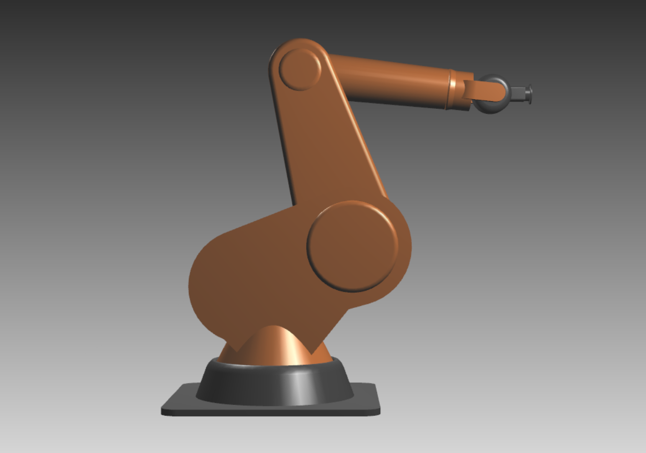
Fig. 28.4 The robot called generic robot.
# Save all the hinges of the robot in a list
hinges = [robot.hinges["bottom"], robot.hinges["bottomMiddle"], robot.hinges["middleTop"],
          robot.hinges["topHead"], robot.hinges["head"], robot.hinges["headPlate"]]

# Lists with PID parameters
# Different parameters can be used for the different joints and the
# parameters can be tuned if desired. Currently lists with 6 identical values.
Kp = [900] * 6
Ki = [200] * 6
Kd = [600] * 6

# List of values for motor inertia and gear ratio.
motorInertia = [0.27, 0.046, 0.036, 0.15, 0.15, 0.18]
gearRatio = [125.0, 171.0, 143.0, 60.0, 67.0, 50.0]

powerLine = agxPowerLine.PowerLine()
sim.add(powerLine)

joints = []
for i in range(0, len(hinges)):
    hinges[i].getMotor1D().setEnable(False)
    engine = agxDriveTrain.Engine()
    engine.setPowerGenerator(agxPowerLine.TorqueGenerator(engine.getRotationalDimension()))
    lookupTable = engine.getPowerGenerator().getPowerTimeIntegralLookupTable()
    engine.setThrottle(1.0)
    engine.setInertia(motorInertia[i])
    powerLine.add(engine)

    actuator = agxPowerLine.RotationalActuator(hinges[i])
    gear = agxDriveTrain.HolonomicGear()
    gear.setGearRatio(gearRatio[i])

    engine.connect(gear)
    gear.connect(actuator)

    joints.append(RobotJoint(hinges[i], lookupTable, Kp[i], Ki[i], Kd[i]))
A controller can then be created. The joints should all be put in a list, that is sent into the controller.
simulation().add(ControlLoop(joints, fullFileName))
Running the tutorial with the square example with the above controller should give the result seen in the figure below.
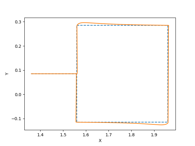
Fig. 28.5 Robot tool position in the x-y-plane. The values are in meters and the dashed line is the reference. The robot follows the straight line to the square, then moves clockwise around the square path.
For more details see data/python/tutorials/RobotControl/tutorial_robot_pid_control.agxPy.