42. Journal Viewer
Note
The Journal viewer is only available under Windows operating system.
Journal Viewer is a Graphical User Interface (GUI) that allows you to play and post-process journals, as shown in Fig. 42.1.

Fig. 42.1 The interface of the Journal Viewer. A journal from a simulation of a curved two-lane conveyor transporting bottles is loaded.
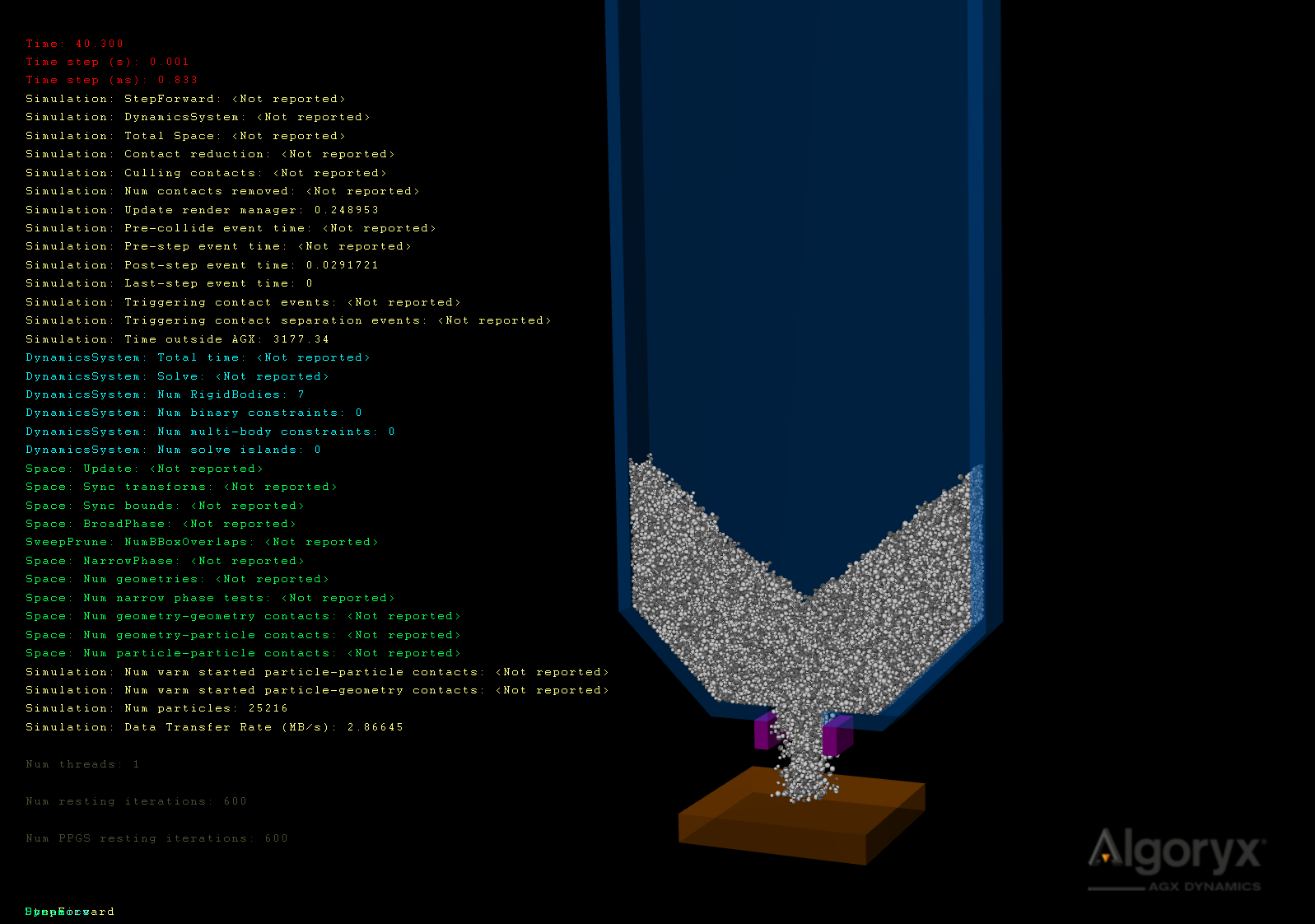
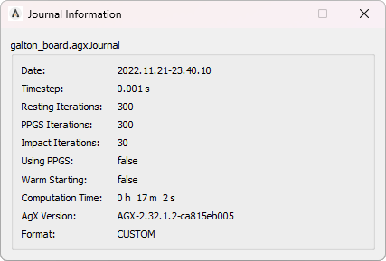
In AGX Dynamics (and Algoryx Momentum), simulation data can be stored in an .agxJournal file. This simulation data file, known as a journal, is a recording of the simulation.
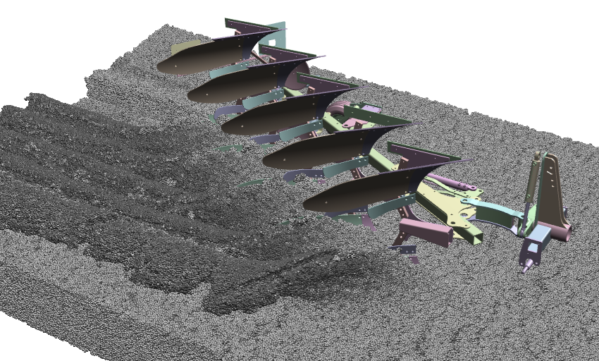
By playing the journal with the Journal Viewer, the saved simulation is displayed similarly to a video, but unlike a traditional video that consists of image frames, this playback uses simulation data, such as object positions, velocities, and other properties. This allows for dynamic viewing from any angle, zooming in or out, and offers post-processing capabilities such as coloring particles based on scalar quantities (e.g., velocity), and much more. Additionally, custom scripts can be appended for tailored post-processing.
In this section, we will describe how to find and use Journal Viewer, including how to load and play a journal, as well as its post-processing features. First, we will describe the key functions and features. Following this, we will detail the specific menu items, explaining how each one contributes to the overall functionality. Lastly, we’ll describe how to create and use custom scripts for tailored post-processing.
42.1. Save Journal
In AGX Dynamics (and Algoryx Momentum), simulation data can be stored in an .agxJournal, which can later be played using the Journal Viewer. This file, referred to as a journal, contains a detailed recording of the simulation, including various data points (object positions, velocities, etc.). To save a journal using AGX Dynamics, you can use agxViewer (see agxViewer). To save a journal, open your terminal, set up your AGX environment, and run the following command:
>> agxviewer <agxScenePath> --journalRecord
where <agxScenePath> is the path to the AGX scene file, which can be either relative to the current directory or an absolute path. This saves the journal to the default journal filename Journal.agxJournal.
For example, to save a journal for the scene located at D:/agx_scenes/excavator_E85_terrain.agxPy, run this command from any directory:
>> agxviewer D:/agx_scenes/excavator_E85_terrain.agxPy --journalRecord
Alternatively, if you are already in the directory D:/agx_scenes/, you can simplify the command:
>> agxviewer excavator_E85_terrain.agxPy --journalRecord
To save the journal to a custom path, either relative to the current directory or an absolute path, use the argument --journalRecordPath followed by the custom path. For example:
>> agxviewer excavator_E85_terrain.agxPy --journalRecord --journalRecordPath excavator_E85_terrain.agxJournal
To explore more options related to journal recording, use the following command:
>> agxviewer --help
42.2. Launch Journal Viewer
The Journal Viewer is located in .../bin/ARCH/, where ARCH corresponds to your system’s architecture. For example, if you are using Windows with a 64-bit architecture, the location would be .../bin/x64/journalViewer.exe.
Additionally, the Journal Viewer can be accessed from the terminal or shell from any folder, similar to how agxViewer is accessed. To do this, open your terminal, set up you AGX environment, type journalViewer, and press Enter. The interface of the Journal Viewer will appear, as shown in Fig. 42.2.

Fig. 42.2 The interface of the Journal Viewer with no journal loaded.
To launch the Journal Viewer and simultanously load a journal, refer to Load journal.
42.3. Load journal
To load a journal, navigate to the main menu (Main > Open File) and select the desired journal file. Once a journal is loaded, the interface will display the simulation, as shown in Fig. 42.3.

Fig. 42.3 A loaded journal of a scene with an E85 excavator.
You can also launch the Journal Viewer and simultaneously load a journal directly from the terminal. To do this, use the following command:
>> journalviewer <journalPath>
where <journalPath> is the path to the journal, which can be either relative to the current directory or an absolute path.
For example, to load the journal located at D:/journals/excavator_E85_terrain.agxJournal, you would run the following command from any directory:
>> journalviewer D:/journals/excavator_E85_terrain.agxJournal
Alternatively, if you are already in the directory D:/journals/, you can simply use:
>> journalviewer excavator_E85_terrain.agxJournal
42.4. Playback
The playback panel of the Journal Viewer, see Fig. 42.4, functions similarly to the controls of a traditional video player.

Fig. 42.4 The playback panel.
Table 42.1 describes the buttons and items found on the playback panel.
ITEM |
DESCRIPTION |
|---|---|
Play/Pause |
Starts the playback of the journal. If playback is active, the play button changes to a pause button. |
Stop |
Stops playback and returns to the beginning of the journal. |
Previous Frame |
Steps backward by N simulation frames, where N is the current frame stride. |
Next Frame |
Steps forward by N simulation frames. |
Decrease Frame Stride |
Reduces the frame stride. Frame stride refers to the number of simulation frames skipped at each playback step. For example, if the frame stride is set to 4, every 4th frame is displayed during playback. |
Increase Frame Stride |
Increases the frame stride. |
Current Frame Stride |
Displays the current frame stride value. |
Current Time |
Shows the current playback time. |
End Time |
Displays the total duration of the journal. |
Loop Journal |
When enabled, the journal replays continuously after reaching the end. |
42.5. Adjusting the viewing window
The viewing window is the area where the simulation and its objects are displayed. Users can adjust the view using the mouse, keyboard, or specific settings. In this section, we describe the available mouse and keyboard commands for interacting with the viewing window.
Table 42.2 lists the mouse commands for manipulating the viewing window.
MOUSE BUTTON |
ACTION |
|---|---|
Left |
Zoom in or out by moving the mouse up or down |
Scroll wheel |
Pan the view horizontally or vertically by moving the mouse in any direction. |
Right |
Rotate the object by moving the cursor in any direction. |
Table 42.3 lists the keyboard commands for manipulating the viewing window.
KEY |
ACTION |
|---|---|
space |
Reset and center view to display all objects. |
b |
Draw statistics (time, timestep, etc.). |
+ |
Increment the clip plane position in the direction of the clip plane normal. |
- |
Decrement the clip plane position in the direction of the clip plane normal. |
p |
Toggle the left side docket (containing Analysis and Coloring). |
Ctrl+1 to Ctrl+6 |
Set the view to the positive/negative direction of a coordinate axis. 1: X, 2: -X, 3: Y, 4: -Y, 5: Z, 6: -Z. |
Ctrl+7 |
Set the view to the normal direction of the clip plane. |
Ctrl++ |
Zoom in with Orthographic View (if orthographic mode is enabled). |
Ctrl+- |
Zoom out with Orthographic View (if orthographic mode is enabled). |
J |
Open a Camera File. |
K |
Save Cameras. The currently stored camera views are saved to an |
H |
Show Views. Opens a panel with the currently stored camera views. |
M |
Store Current Camera. |
PgUp |
Next Camera. Selects the next camera view stored. |
PgDown |
Previous Camera. Selects the previous camera view stored. |
G |
Debug Rendering. |
O |
Standard Rendering. |
Home |
Mesh Rendering > Collision Mesh. |
Ins |
Mesh Rendering > Render Mesh |
F12 |
Take screenshot. The image is saved to the directory of the journal. |
e |
Plays/pauses playback. |
l |
Sets the light source in the direction of the current view. |
42.6. Cameras
The Cameras menu allows you to store different camera views, either temporarily or permanently in a file, making it easy to switch between saved views. To save a camera view, first adjust the viewing window to your desired position (refer to Adjusting the viewing window for details). Then, select Store Current Camera (shortcut: M) to add the current view to an internal list. You can repeat this process by adjusting the viewing window and selecting Store Current Camera again to save multiple views.
To view the list of saved camera views, select Show Views, which will display the list on the right side of the screen. To navigate between stored views, use Next Camera (PgUp) to cycle forward through the list or Previous Camera (PgDown) to go back.
To save your list of camera views to a file, select Save Cameras (shortcut: K). This will open a file dialog where you can save the views as a .cfg file in a folder of your choice. To load a previously saved camera views file, select Open Camera File (shortcut: J) and choose the desired file.
Note
If you save a camera file in the same folder as a journal with the same name as the journal (except for the file extension), then, by loading the journal, the camera file will automatically be loaded.
42.7. Media
The Media menu offers options to save a video file of the journal and capture screenshots.
To save a video, start by loading the desired journal and adjusting the size of the viewing window. Keep in mind that the window size directly affects the video’s resolution; for instance, a full-screen viewer will result in a larger video than a smaller window. Next, select Video Generation Settings (shortcut: V), which opens the window shown in Fig. 42.5.
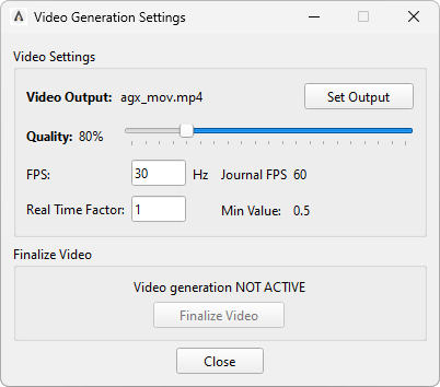
Fig. 42.5 The Video Generation Settings window.
In the settings window, start by clicking Set Output to choose the filename and directory for the video. You can adjust the video quality using the quality slider. FPS determines the Frames Per Second of the video. The journal’s current FPS is displayed to the right. You’ll also set the Real Time Factor (RTF), which controls the playback speed relative to real time:
RTF = 1. The video will play in real time. A 10-second simulation will result in a 10-second video.
RTF > 1. The video will play faster than real time. For example, with an RTF of 2, a 10-second simulation will produce a 5-second video.
RTF < 1. The video will play slower than real time. For instance, with an RTF of 0.5, a 10-second simulation will produce a 20-second video.
Once the settings are configured, select Close.
To begin recording, ensure the journal is paused, then select Capture Video (shortcut: C) from the Media menu. A red “Recording Video” message will appear above the playback panel. As the simulation progresses (either by playing or advancing frame by frame), the content shown in the main window will be recorded. You can pause and resume recording as needed, and adjust the camera view during the recording. Be careful not to use the Stop button, as this will reset the playback. Once you have recorded the desired content, pause the video, return to Video Generation Settings, and select Finalize Video to save the recording.
To take a screenshot, select Take Screenshot (shortcut: F12). This captures an image of the current frame and saves it to the journal’s directory. Similar to video generation, the screenshot will reflect the current size of the viewing window.
42.8. Analysis (tab)
The Analysis tab located in the left side docket is shown in Fig. 42.6. It provides a range of features designed to enhance the visualization and exploration of scenes, and carry out measurements and analyzes. It allows users to isolate specific regions, manipulate views, and obtain detailed data about objects or areas of interest. The features are described in the section below.
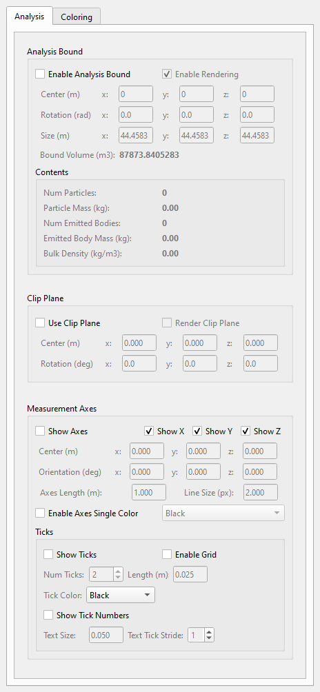
Fig. 42.6 The analysis tab.
42.8.1. Analysis Bound
The Analysis Bound function is available within the Analysis tab, as shown in Fig. 42.7.
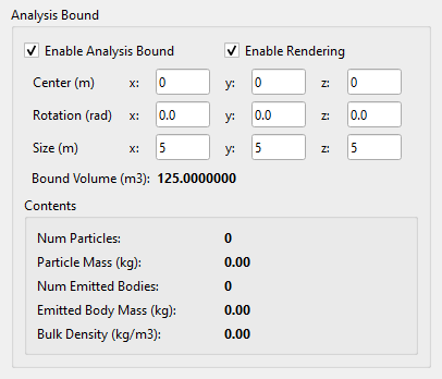
Fig. 42.7 The Analysis Bound Tab.
This feature allows users to define a rectangular region in the scene with customizable size, position, and orientation. Enable Analysis Bound activates or deactivates this region, while Enable Rendering toggles the visual display of the Analysis Bound, shown as a blue rectangle. Once enabled, statistical data for the defined region are displayed in the Contents panel. An example with and without the Analysis Bound is illustrated in Fig. 42.8.

Fig. 42.8 A scene with a CAT365 excavator about to dig. (a) No analysis bound enabled. (b) Analysis bound enabled.
The settings and data for Fig. 42.8 are shown in Fig. 42.9.

Fig. 42.9 The analysis bound settings for Fig. 42.8. (a) No analysis bound enabled. (b) Analysis bound enabled.
In this example, the Analysis Bound has been configured to match the excavator’s digging area. By analyzing the Contents panel in Fig. 42.9 (b), we can derive useful data such as the number of particles (246946) and the bulk density (1509 kg/m³) within the defined region.
42.8.2. Clip Plane
The Clip Plane function is available in the Analysis tab, as shown in Fig. 42.10.
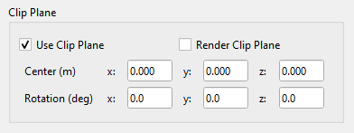
Fig. 42.10 The Clip Plane panel.
This feature introduces an xz-plane that slices through the scene, rendering all objects with negative y-coordinates invisible, effectively “clipping” those portions. The position and orientation of the Clip Plane can be adjusted by changing its center or rotating it, allowing users to clip the scene in any desired configuration. To active the feature, check Use Clip Plane. To activate the visual display of the Clip Plane, which appears as a red rectangle with diagonal lines, check Render Clip Plane. The point where these lines intersect represents the center of the Clip Plane, aiding in precise positioning and orientation.
A usage example is shown in Fig. 42.11.

Fig. 42.11 An CAT365 excavator in the process of digging. Particle coloring by velocity. Particle color interval: [0, 1] m/s. (a) Clip Plane not enabled. (b) Clip Plane enabled and positioned to split the scene along the length of the digging area. (c) Clip Plane enabled, centered at the bucket, and rotated 30 degrees about the vertical axis.
In Fig. 42.11 (a), the soil dynamics are obscured by particles and the excavator bucket, demonstrating the need for the Clip Plane. In contrast, Fig. 42.11 (b) reveals the dynamics within the soil and inside the bucket. Finally, Fig. 42.11 (c) shows the effect of rotating the Clip Plane for a different view angle.
42.8.3. Measurement Axes
The Measurement Axes function can be accessed from the Analysis tab, as shown in Fig. 42.12.
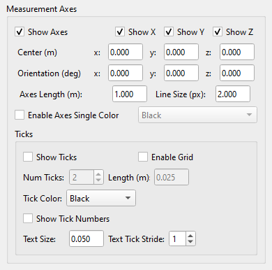
Fig. 42.12 The Measurement Axes panel.
This feature provides a customizable coordinate system that can be moved, rotated, and customized.
To activate the coordinate system, check Show Axes, which displays a red x-axis, a green y-axis, and a blue z-axis. Individual axes can be shown or hidden by toggling Show X, Show Y, or Show Z. The coordinate system can be repositioned by adjusting the Center (m) values for x, y, and z, with the default position at (0,0,0) representing the scene’s origin. The axes length and line thickness can be adjusted using Axes Length (m) and Line Size (px), respectively. Additionally, you can change the default colors to a single one using Enable Axes Single Color, which is helpful when the default colors blend into the scene.
Enabling Show Ticks adds tick markers to the axes, and the number and length of these ticks can be adjusted via Num Ticks and Length (m). To display grids, check Enable Grid, and customize tick colors using Tick Color. You can also show tick numbers by enabling Show Tick Numbers, with options to adjust the font size (Text Size) and change how often numbers appear by specifying a Text Tick Stride. The default stride value of 1 labels every tick, while higher values (e.g., 2 or more) reduce the frequency of numbered ticks.
An example of Measurement Axes usage is provided in Fig. 42.13.

Fig. 42.13 A recirculation conveyor with curved walls transporting barrels. (a) Measurment axes disabled. (b) Measurment axes enabled. Axes length: 1.5 m. Line size: 4px. (c) Close-up view of (b). (d) Same as (c), but with Show Ticks and Enable Grid checked, and Num Ticks set to 3.
42.9. Coloring (tab)
The Journal Viewer provides a variety of tools for coloring and post-processing granular particles, accessible through the Coloring tab in the left side docket. This tab contains two sub-tabs: Particle Color and Particle Primitives. Below is a brief overview of each:
Particle Color: Allows particles to be colored based on scalar values such as velocity, displacement, or radius.
Particle Primitives: Provides visualization of particle dynamics using trajectories and contact networks.
These two sub-tabs are described in the following sections.
42.9.1. Particle Color
The Particle Color tab is displayed in Fig. 42.14.

Fig. 42.14 The particle color tab.
The central feature of this tab is to color particles based on scalar quantities such as velocity, displacement, or radius.
The Alpha value, found under Alpha Settings, controls the opacity of particles when Alpha Sprites are enabled (see Particle Shader).
The dropdown list titled Scalar coloring provides a range of scalar quantities for coloring. If Limit to Analysis Bound is checked, only particles within the analysis bound will be colored. The colormap is defined by specifying minimum (Min) and maximum (Max) values. Particles at or below the minimum are colored blue, while those at or above the maximum are colored red. Particles with intermediate values will transition smoothly through a gradient of colors, as shown in Fig. 42.15.
The Particle Render Filter applies a threshold to the coloring, meaning only particles exceeding a selected quantity will be colored. For an example, refer to Velocity.
In the Legend Settings, the color legend, which reflects the Min-Max color interval, can be customized in terms of size, orientation (horizontal or vertical), and placement. An example legend for displacement, ranging from -2 to 4 m, is shown in Fig. 42.15.

Fig. 42.15 An example legend for displacement. Interval: [-2, 4] m.
42.9.1.1. Contact Force
This feature colors particles based on the magnitude of the contact forces acting on them. Visualizing particles in this way helps identify areas of high stress or compression, which is useful for analyzing how forces are distributed in granular systems. For instance, it can highlight potential breakage points in materials such as powders or soils under pressure. To use this feature, select Contact Force from the Scalar coloring dropdown. An example is shown in Fig. 42.16.

Fig. 42.16 A tractor tyre on a bed of particles. Contact force coloring interval: [0, 100] Nm.
In the example (Fig. 42.16), the highest contact forces are concentrated beneath the tire and spread outward from the tire-soil interface. This pattern is characteristic of granular materials like soil, where forces are transmitted through networks of interconnected force chains. These force chains distribute the load unevenly, creating regions of high stress extending from the point of contact.
42.9.1.2. Displacement
Coloring particles by displacement reveals how far they have moved from their initial positions, making it useful for identifying deformation patterns or flow paths over time. This feature is particularly valuable for studying pile formations, static regions, or other processes involving particle rearrangement.
To use this feature, first navigate to the desired time in the simulation. Then, select Displacement from the Scalar coloring dropdown, which establishes the reference positions of the particles at that specific moment. Next, set the desired coloring interval. As the journal progresses, particles will be colored according to how far they have moved from their reference positions, representing their displacement. An example is shown in Fig. 42.17.

Fig. 42.17 A tall silo with an outlet. Displacement coloring interval: [0, 2] m. (a) The reference time at which the outlet is opened; (b) 1.5 s after the outlet has opened; (c) 4 s after the outlet has opened.
In Fig. 42.17 (a), all particles are blue, indicating a displacement of 0 m, as this is the reference time. In Fig. 42.17 (b), 1.5 seconds later, displacement is concentrated in a semi-elliptic region aligned with the outlet, suggesting this area experiences the most flow. By Fig. 42.17 (c), 4 seconds after opening the outlet, the displacement has expanded, forming a red cylinder through the outlet, extending halfway up the silo. Above this region, a gradient of orange, yellow, and green indicates decreasing displacement, showing non-uniform flow. Meanwhile, particles near the bottom walls remain blue, indicating they are static.
42.9.1.3. Height X (Y, Z)
Coloring particles based on their height along a specific axis provides useful insights into the spatial distribution and layering of particles. It can also help identify particles that exceed a critical height, such as in a silo scenario. To use this feature, select Height X, Height Y, or Height Z from the Scalar coloring dropdown. An example is shown in Fig. 42.18.

Fig. 42.18 A tractor driving on a bed of particles. Height (Y) coloring interval: [1.9, 2.5] m.
In Fig. 42.18, particles are colored by their height along the Y axis, as gravity acts in this direction. This height-based coloring provides an intuitive way to differentiate undisturbed soil from areas affected by the tractor’s movement. In this example, the surface of the soil is mostly green, while the tracks left by the tractor are identifiable by their red color.
42.9.1.4. Kinetic Energy
Kinetic energy coloring offers valuable insights into how energy is distributed among particles, helping to track energy dissipation within the system. This is particularly useful for analyzing collisions, identifying areas where energy is concentrated or lost, and optimizing process efficiency. To use this feature, select Kinetic Energy from the Scalar coloring dropdown. An example is shown in Fig. 42.19.

Fig. 42.19 A heavy wall pipe section falling onto a particle bed. Kinetic energy coloring interval: [0, 0.01] J. (a) Prior to impact. (b) About 5 ms after impact. (b) About 25 ms after impact.
We note in Fig. 42.19 (a) that just after impact, the particles just beneath the pipe has absorbed a relatively large amount of kinetic energy. In Fig. 42.19 (b), a short time later, this energy has dissipated and also been transmitted to more distant regions.
In Fig. 42.19 (a), prior to impact, the kinetic energy is essentially zero, as the particles are static. By Fig. 42.19 (b), 5 ms after impact, the particles directly beneath the pipe absorb a significant amount of kinetic energy from the pipe section. By Fig. 42.19 (c), 25 ms after the impact, this energy has begun to dissipate and spread to surrounding regions.
42.9.1.5. Velocity
Coloring particles by velocity helps visualize dynamic regions within the system. This method highlights areas of rapid motion or flow, making it useful for assessing granular flows, detecting eddies, or evaluating mixing efficiency. The coloring is based on the magnitude of the velocity vector. To use this feature, select Velocity from the Scalar coloring dropdown. An example is shown in Fig. 42.20.

Fig. 42.20 A rotary drum with pellets modelled as granular particles. Velocity coloring interval: [0, 1] m/s. (a) No filter threshold. (b) Filter threshold: 0.5 m/s.
In Fig. 42.20 (a), the highest velocities are observed on the surface of the material, while the velocity is lowest inside the bulk. In Fig. 42.20 (b), a filter threshold of 0.5 m/s has been applied using the Particle Render Filter, with Velocity selected for filtering. This renders particles below the threshold invisible, effectively isolating regions of faster movement.
42.9.1.6. Radius
This feature colors the particles according to their radii. The radius coloring feature is particularly useful for identifying particle segregation, which is the phenomenon in which granular particles of different sizes separate into distinct regions. This allows users to easily visualize how particles of specific radii migrate and cluster in certain areas of the system over time. To use this feature, select Radius from the Scalar coloring dropdown. An example is shown in Fig. 42.21.

Fig. 42.21 A rotary drum with pellets modelled as granular particles. Radius coloring interval: [0.005, 0.01] m. Particles of radius 0.005, 0.075, and 0.01 m are blue, green, and red, respectively. (a) The initial state; (b) Shortly after the drum has started to rotate; (c) After 30 seconds of rotation.
In Fig. 42.21 (b), shortly after the drum starts rotating, particles of different radii are more or less uniformly distributed. However, as the drum continues to rotate, Fig. 42.21 (c) shows that smaller particles congregate in the center of the bulk.
42.9.2. Particle Primitives
The Particle Primitives tab, as shown in Fig. 42.22, provides post-processing tools that visualize particle dynamics using lines and curves. The available features are Trajectory Lines and Contact Network, which help illustrate the movement and interactions of particles in the system.

Fig. 42.22 The particle primitives tab.
42.9.2.1. Trajectory Lines
The Trajectory Lines feature analyzes particle motion and visualizes it by drawing trajectory lines that trace the paths of the particles. This feature offers two key settings:
Number of positions: This setting defines how many previous particle positions are used to create the trajectory line. A trajectory is constructed by connecting these past positions with straight segments. If set to 2, the trajectory consists of a single straight line. With values of 3 or higher, the lines become more complex, capturing more detailed particle movement.
Samples: This setting determines the percentage of particles to include when rendering trajectory lines.
An example is shown in Fig. 42.23.

Fig. 42.23 A rotary drum with pellets modelled as granular particles. (a) No particle trajectories rendered. (b) Particle trajectories rendered. Number of positions: 8. Samples: 4%.
42.9.2.2. Contact Network
The Contact Network feature allows users to visualize all contact forces between particles, represented as lines connecting them. It is similar to the Contact Force coloring option (see Contact Force), but it additionally provides a geometric representation of the forces.
To use this feature, enable Render Contact Network in the Contact Network panel and specify the Min Force (N) and Max Force (N) values. These values work similarly to the Min and Max settings used in Scalar coloring. When rendering the Contact Network, it may be helpful to disable Render Particles at the top of the Particle Primitives tab for a clearer view of the network. An example is shown in Fig. 42.24.

Fig. 42.24 A tyre on a particle soil bed. (a) Contact Network not rendered. Render Particles enabled. (b) Contact Network rendered. Min Force: 0 N. Max Force: 100 N. Render Particles disabled.
42.18. Custom Scripting
The Journal Viewer allows for the attachment of custom Python scripts, enabling custom post-processing capabilities.
To attach a single Python script, use the command line argument --attachScript <filename>. To make all Python modules in a directory available, use the command line argument --addCustomScriptPath <path>. You can view all available command line arguments by executing:
>> journalViewer --help
Examples of using both --attachScript <filename> and --addCustomScriptPath <path> are provided in the sections below.
42.18.1. Attach Script
To attach a custom Python script, my_custom_script.py, to a journal, my_journal.agxJournal, run the following terminal command:
>> journalViewer my_journal.agxJournal --attachScript my_custom_script.py
Let’s illustrate this with an example. Consider the scene shown in Fig. 42.35.

Fig. 42.35 The initial state of a rotating drum with particle pellets. The coordinate system is displayed using Measurement Axes (see Measurement Axes).
To visually inspect the mixing dynamics and efficiency of the pellets in the drum, we can color the particles in two groups: the left half in one color, and the right half in another. We can implement this functionality using a custom script, as described in Code snippet 1 - ParticleColorer.py.
Since the drum is centered at x=0, we can divide the particles based on their position. The script defines a class ParticleColorer, which listens to each simulation time step. After a certain time (TIME_TO_COLOR, set to 4 seconds), the particles are grouped based on their x-coordinate. The IDs of particles in the right half (x >= 0) are stored in one variable, and the IDs of particles in the left half (x <= 0) in another. These variables are assigned once. Then, at each time step, the particles in the right group are colored with one color (COLOR_A, set to purple), and those in the left group with another (COLOR_B, set to yellow).
The complete script is provided in Code snippet 1 - ParticleColorer.py. The journal filename is rotary_drum.agxJournal and we place ParticleColorer.py in the same folder as the journal. To apply the script, execute the following command in the terminal:
>> journalViewer rotary_drum.agxJournal --attachScript ParticleColorer.py
The result is shown in Fig. 42.36.

Fig. 42.36 The evolution of the granular material with ParticleColorer.py attached.
(a) Time: 4 s. (b) Time: 7 s. (c) Time: 10 s. (d) Time: 15 s.
import numpy as np
import agxSDK
import agxPython
from agxPythonModules.utils.numpy_utils import BufferWrapper

TIME_TO_COLOR = 4  # Time to start coloring
COLOR_A = [0.502, 0, 0.502, 1]  # Purple
COLOR_B = [1, 1, 0, 1]  # Yellow

def buildViewerScene() -> None:
    '''Build the viewer scene and add the particle colorer to the simulation.'''
    sim = agxPython.getContext().environment.getSimulation()
    particle_colorer = ParticleColorer(sim)
    sim.add(particle_colorer)

class ParticleColorer(agxSDK.StepEventListener):
    def __init__(self, sim: agxSDK.Simulation) -> None:
        super().__init__()
        self.sim: agxSDK.Simulation = sim
        self.particle_ids_x_geq_0: Optional[np.ndarray] = None
        self.particle_ids_x_lt_0: Optional[np.ndarray] = None

    def post(self, time: float) -> None:
        '''Executed after each simulation step.'''
        if time >= TIME_TO_COLOR:
            if self.particle_ids_x_geq_0 is None or self.particle_ids_x_lt_0 is None:
                self.particle_pos = BufferWrapper(self.sim, 'Particle.position').array
                self.particle_id_to_index = BufferWrapper(self.sim, 'Particle._idToIndex').array
                self.particle_color = BufferWrapper(self.sim, 'Particle.color').array
                self.particle_ids_x_geq_0, self.particle_ids_x_lt_0 = \
                    self.get_particle_ids_for_coloring()
            self.color_particles()

    def color_particles(self) -> None:
        '''Color particles based on their IDs.'''
        indices_x_geq_0 = self.particle_id_to_index[self.particle_ids_x_geq_0]
        indices_x_lt_0 = self.particle_id_to_index[self.particle_ids_x_lt_0]
        self.particle_color[indices_x_geq_0] = COLOR_A
        self.particle_color[indices_x_lt_0] = COLOR_B

    def get_particle_ids_for_coloring(self) -> tuple[np.ndarray, np.ndarray]:
        '''
        Get the IDs of particles based on their x-coordinate.
        particle_ids_x_geq_0: particles with x >= 0
        particle_ids_x_lt_0:  particles with x < 0
        '''
        particle_index_to_id = np.argsort(self.particle_id_to_index[:, 0])
        particle_ids_x_geq_0 = particle_index_to_id[np.where(self.particle_pos[:, 0] >= 0)[0]]
        particle_ids_x_lt_0 = particle_index_to_id[np.where(self.particle_pos[:, 0] < 0)[0]]
        return particle_ids_x_geq_0, particle_ids_x_lt_0
Code Snippet 1 - ParticleColorer.py
42.18.2. Add Custom Scripts Path
In the example from the previous section, where we colored particles in two distinct colors, it was sufficient to contain all the custom scripting in a single script, as the code was relatively short. However, for more extensive post-processing, it can be more convenient to divide the script across several files for better clarity. This approach can be utilized in the Journal Viewer by using the --addCustomScriptPath <Path> argument.
To attach a custom Python script, my_custom_script.py, to a journal, my_journal.agxJournal, while also making the modules in D:/my_custom_utils/ accessible to my_custom_script.py, execute the following terminal command:
>> journalViewer my_journal.agxJournal --attachScript my_custom_script.py --addCustomScriptPath D:/my_custom_utils/
Let’s illustrate this with an example. We will reuse the functionality from the previous section, where particles were divided at x=0 into left and right collections. Additionally, we will add functionality to store the centers of mass for both collections and save this data into a .json file for later plotting. We will break out the ParticleColorer class into a separate file, particle_colorer.py, create a new class, CenterOfMassAnalyzer, to handle center of mass calculations in CenterOfMassAnalyzer.py, and create a class, ParticlePostProcessor, responsible for managing both previous classes in ParticlePostProcessor.py. We place ParticleColorer.py and CenterOfMassAnalyzer.py in D:/particle_post_processor_utils/, while placing ParticlePostProcessor.py in the same directory as the journal rotary_drum.agxJournal. (See Code snippet 3 - ParticlePostProcessor.py, Code snippet 4 - ParticleColorer.py, and Code snippet 5 - CenterOfMassAnalyzer.py for details.)
Navigate to the directory where the journal is located. To execute the post-processing script, use the following terminal command:
>> journalViewer rotary_drum.agxJournal --attachScript ParticlePostProcessor.py --addCustomScriptPath D:/particle_post_processor_utils/
A key feature here is that --addCustomScriptPath D:/particle_post_processor_utils/ makes the modules in that directory available to ParticlePostProcessor.py. By studying Code snippet 3 - ParticlePostProcessor.py, we can see that this script imports the ParticleColorer and CenterOfMassAnalyzer classes from the files in the directory D:/particle_post_processor_utils/.
When running the above command, the particle coloring works as described in the previous section. The new addition is the creation of a .json file that contains the center of mass positions for both particle collections as a function of time. An (abbreviated) version of this file is shown in Code snippet 2 - com_data.json
{
    "time": [
        4.0000000000002185,
        4.033333333333557,
        ...
    ],
    "pos_left": [
        [
            -0.16945233435221013,
            2.187992830899125e-05,
            -0.40797553851422996
        ],
        [
            -0.16945324192040673,
            2.1973870151488706e-05,
            -0.40797750815201633
        ],
        ...
    ],
    "pos_right": [
        [
            0.16720595499825752,
            -3.968564056495067e-05,
            -0.4074566484874103
        ],
        [
            0.16720676731927853,
            -3.968090879135949e-05,
            -0.4074585782608062
        ],
        ...
    ]
}
Code Snippet 2 - com_data.json
This .json data can be plotted using various programs. A plot generated by a Python script is shown in Fig. 42.37.

Fig. 42.37 Center of mass coordinates vs. time for the two particle collections in Fig. 42.35. Plotted using the data in Code snippet 2 - com_data.json.
As shown in Fig. 42.37, the mass centers in the xz-plane move in elliptical trajectories with decreasing amplitudes. This behavior is expected: as the two collections mix, their centers of mass converge, leading to the decays. Additionally, both y coordinates remain almost constant, which is also expected, as the drum’s axis lies along the y-axis, and there is no significant flow in the axial direction.
import numpy as np
import agxSDK
import agxPython
from agxPythonModules.utils.numpy_utils import BufferWrapper
from ParticleColorer import ParticleColorer
from CenterOfMassAnalyzer import CenterOfMassAnalyzer

settings = {
    "time_to_start": 4,  # Start time for coloring and analysis
    "time_to_end": 44,  # End time for coloring and analysis
    "color_A": [0.502, 0, 0.502, 1],  # Purple
    "color_B": [1, 1, 0, 1],  # Yellow
    # Path to save center of mass data
    "path_to_data_file_to_save": "D:/particle_post_processor_utils/com_data.json"
}

def buildViewerScene() -> None:
    '''Build the viewer scene and add particle post-processor.'''
    sim = agxPython.getContext().environment.getSimulation()
    particle_post_processor = ParticlePostProcessor(sim, settings)
    sim.add(particle_post_processor)

class ParticlePostProcessor(agxSDK.StepEventListener):
    def __init__(self, sim: agxSDK.Simulation, settings: dict) -> None:
        super().__init__()
        self.sim = sim
        self.settings = settings
        self.particle_colorer = ParticleColorer(self.settings)
        self.center_of_mass_analyzer = CenterOfMassAnalyzer(self.settings)
        self.has_saved_data = False
        self.particle_ids_x_geq_0 = None
        self.particle_ids_x_lt_0 = None

    def post(self, time: float) -> None:
        '''Executed after each simulation step.'''
        if self.settings["time_to_start"] < time <= self.settings["time_to_end"]:
            if self.particle_ids_x_geq_0 is None or self.particle_ids_x_lt_0 is None:
                self.initiate_buffers()
                self.particle_ids_x_geq_0, self.particle_ids_x_lt_0 = \
                    self.particle_colorer.get_particle_ids_for_coloring(
                        self.particle_pos,
                        self.particle_id_to_index)
            self.particle_colorer.color_particles(
                self.particle_color,
                self.particle_id_to_index,
                self.particle_ids_x_geq_0,
                self.particle_ids_x_lt_0)
            self.center_of_mass_analyzer.store_data(
                time,
                self.particle_pos,
                self.particle_mass,
                self.particle_id_to_index,
                self.particle_ids_x_geq_0,
                self.particle_ids_x_lt_0)
        elif time > self.settings["time_to_end"] and not self.has_saved_data:
            self.center_of_mass_analyzer.save_data()
            self.has_saved_data = True

    def initiate_buffers(self) -> None:
        '''Initialize simulation buffers for particles.'''
        self.particle_pos = BufferWrapper(self.sim, 'Particle.position').array
        self.particle_id_to_index = BufferWrapper(self.sim, 'Particle._idToIndex').array
        self.particle_mass = BufferWrapper(self.sim, 'Particle.mass').array
        self.particle_color = BufferWrapper(self.sim, 'Particle.color').array
Code Snippet 3 - ParticlePostProcessor.py
import numpy as np

class ParticleColorer():
    def __init__(self,  settings: dict) -> None:
        self.settings: dict = settings

    def color_particles(self, particle_color, particle_id_to_index, particle_ids_x_geq_0, particle_ids_x_lt_0) -> None:
        '''Color particles based on their IDs.'''
        indices_x_geq_0 = particle_id_to_index[particle_ids_x_geq_0]
        indices_x_lt_0 = particle_id_to_index[particle_ids_x_lt_0]
        particle_color[indices_x_geq_0] = self.settings["color_A"]
        particle_color[indices_x_lt_0] = self.settings["color_B"]

    def get_particle_ids_for_coloring(self, particle_pos, particle_id_to_index) -> tuple[np.ndarray, np.ndarray]:
        '''
        Get the IDs of particles based on their x-coordinate.
        particle_ids_x_geq_0: particles with x >= 0
        particle_ids_x_lt_0:  particles with x < 0
        '''
        particle_index_to_id = np.argsort(particle_id_to_index[:, 0])
        particle_ids_x_geq_0 = particle_index_to_id[np.where(particle_pos[:, 0] >= 0)[0]]
        particle_ids_x_lt_0 = particle_index_to_id[np.where(particle_pos[:, 0] < 0)[0]]
        return particle_ids_x_geq_0, particle_ids_x_lt_0
Code Snippet 4 - ParticleColorer.py
import numpy as np
import json

class CenterOfMassAnalyzer():
    def __init__(self, settings: dict) -> None:
        self.settings = settings
        self.data = {
            "time": np.array([]),  # Array to store time steps
            "pos_left": np.empty((0, 3)),  # Empty array for left side positions
            "pos_right": np.empty((0, 3))  # Empty array for right side positions
        }

    def store_data(self, time, particle_pos, particle_mass, particle_id_to_index, particle_ids_x_geq_0, particle_ids_x_lt_0) -> None:
        '''Store the center of mass for left and right particle collections.'''
        center_of_mass_left = self.get_center_of_mass(particle_pos, particle_mass, particle_id_to_index, particle_ids_x_lt_0)
        center_of_mass_right = self.get_center_of_mass(particle_pos, particle_mass, particle_id_to_index, particle_ids_x_geq_0)
        self.data["time"] = np.append(self.data["time"], time)
        self.data["pos_left"] = np.vstack([self.data["pos_left"], center_of_mass_left])
        self.data["pos_right"] = np.vstack([self.data["pos_right"], center_of_mass_right])

    def save_data(self) -> None:
        '''Save center of mass data to a JSON file.'''
        data_to_save = {
            "time": self.data["time"].tolist(),
            "pos_left": self.data["pos_left"].tolist(),
            "pos_right": self.data["pos_right"].tolist()
        }
        with open(self.settings["path_to_data_file_to_save"], 'w') as f:
            json.dump(data_to_save, f, indent=4)
        print(f'Data saved to {self.settings["path_to_data_file_to_save"]}')

    def get_center_of_mass(self, particle_pos, particle_mass, particle_id_to_index, particle_selected_ids) -> np.ndarray:
        '''Calculate the center of mass for the selected particles.'''
        particle_selected_indices = particle_id_to_index[:, 0][particle_selected_ids]
        particle_selected_pos = particle_pos[particle_selected_indices]
        particle_selected_mass = particle_mass[particle_selected_indices]
        total_mass = particle_selected_mass.sum()
        particle_selected_pos_weighted = (particle_selected_pos[:, :3] * particle_selected_mass).sum(axis=0)
        return particle_selected_pos_weighted / total_mass
Code Snippet 5 - CenterOfMassAnalyzer.py

