51. Matlab/Simulink plugin
AGX Dynamics has a plugin to Matlab and Simulink, which can be used in order to run AGX as a co-simulation. This is done via a predefined AGX-block which appears in the Simulink library after installation of AGX, and which can easily be modified to create and load your own AGX simulations.
Furthermore, a lower level Matlab coupling is provided.
The Matlab/Simulink plugin is limited to Microsoft Windows operating systems. It has been tested on Windows 10 64bit and Matlab version R2018b.
If your AGX-license does not include a license for the Matlab/Simulink plugin, then please contact Algoryx Simulation for an evaluation license.
Technically, the Simulink coupling is done via an S-function, and the Matlab coupling via a mex-function. Both need to be explicitly compiled as shown below.
Note
To properly run AGX Dynamics inside of Matlab/Simulink. You need to ensure the runtime environment variables is correctly setup. For more information see Section 5.2.1
51.1. Installation
Both the Simulink S-function and the Matlab mex-function source code must be compiled prior to using the AGX functionality inside Simulink/Matlab. All the source code can be found in the following directory:
<agx-dir>/data/Matlab/src
51.1.1. Manual Installation
During the installation process, the following file will be run to register the AGX path to Matlab’s search path, and to compile the s-function and the mex file within Matlab:
<agx-dir>/data/Matlab/addAgXToMatlabAndSimulink.cmd
You can run this file manually (by double-clicking on it).
Attention
The install/uninstall scripts will ask for administrative rights to ensure that it can write in the AGX installation path.
In order to remove the AGX path from Matlab’s search path and to remove the compiled s-function and mex file, the uninstaller will run
<agx-dir>/data/Matlab/removeAgXFromMatlabAndSimulink.cmd
Run this file manually (by double-clicking on it).
51.1.2. Compilation of s-function and mex file
When running the addAgXToMatlabAndSimulink.cmd script the Matlab mex-command will be called in order to compile the source files to the s-function and the mex-function.
These source files are:
Filename |
Purpose |
|---|---|
<agx-dir>/data/Matlab/src/agx_sfun.c |
Code file for Simulink s-function. |
<agx-dir>/data/Matlab/src/agx.c |
Code file for Matlab mex-function. |
The Matlab mex-command is not a compiler in itself, but rather calls a compiler which has been assigned to it. The first time the command is called (which might be now when you install AGX), a compiler has to be chosen from the Matlab prompt by following the instructions there.
A compiler called lcc comes with most Matlab versions on windows, and the two files named above compile fine with it.
Another possible, free compiler under Windows is Microsoft Visual C++ 2015, or its free community version. You might need to restart Matlab in order to find the newly installed compiler.
You can always change the default compiler for Matlab’s mex-command by running mex –setup in the Matlab prompt and following the instructions there.
51.1.3. Manual compilation
The Matlab (agx.c) and Simulink (agx_sfun.c) code can manually be compiled from within Matlab with the following command:
>     cd <AGX-dir>/data/Matlab/src
>     mex agx.c
>     mex agx_sfun.c
Note
If you need to compile with debug information, use the mex –g command.
51.2. Limitation
Within one Matlab session, AGX can be used either only from Simulink using the s-function, or only from Matlab using the mex function. Using the two after each other or next to each other in the same Matlab session is not recommended.
51.3. Starting AGX from Simulink
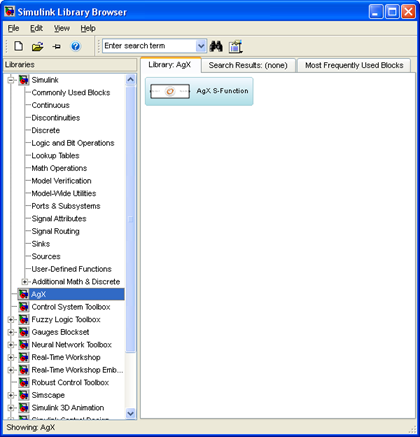
After a successful installation, an AGX-library is going to appear in your Simulink library browser.

Fig. 51.1 AGX-block in Simulink library view.
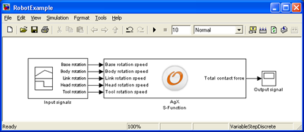
Simply drag a block from there into your model and connect its input and output ports. The simulation is ready to run.

Fig. 51.2 AGX-block in model
Note
There can only be one AGX-block per model. You will get a warning when pressing play in Simulink if you have more than one AGX-block per model.
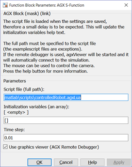
You can modify the block by double-clicking on it.

Fig. 51.3 Modifying the AGX block.
- The following changes can be made:
Script file (full path):
Contains the AGX script-file: It is an .py/.agxPy (Python) script (a script file with AGX commands) which setup the simulation and the coupling between AGX and Simulink. To learn more, look at the sample scripts in <agx-dir>dataMatlabscripts.
Initialization variables:
An array of values to initialize the scene. The length and meaning of the scalars depend on the scene. Descriptions of the parameters are shown in the above the field. If the wrong number of arguments is given, all are set to zero (and a message about that will be sent to the Matlab prompt). Otherwise, after pressing ‘Ok’, the initialization output will be written to the Matlab variable agx_init_output.
Time step:
The simulation time step. AGX uses an internal fixed-size stepper whose time step you can set here.
Use graphics viewer (3D Window with the simulation visualization):
Enables a 3D viewer which render the simulation scene using agxViewer.exe. Using graphics might slow down the simulation.
By checking this box, the viewer will run in the same process as Matlab. For stability reasons we instead strongly recommend that you instead start the viewer prior to Matlab.
This will ensure the viewer run in a separate process. The AGX Dynamics block will automatically detect the running viewer and will not start another one. For more information see Section 51.5
Note
The Help-button gives not only useful help, but also links to a few premade examples which you might want to inspect!
After saving the settings in the block (via Ok/Apply), the AGX script-file will be reloaded. This is necessary in order to adapt the number of ports in the block to the ones in the new or modified script-file.
51.4. Starting AGX from Matlab
An AGX simulation can be controlled from Matlab using the
<result> = agx(<command>, arguments)
Available commands are:
Command |
Description |
|---|---|
load |
Load and initialize a new simulation from a specified AGX script file. |
step |
Take one simulation step |
visual |
Enable/Disable the 3D rendering window |
The syntax for loading an AGX-simulation in Matlab is:
>> [sizeInitInput, initOutput, sizeStepInput, sizeStepOutput] = agx('load', <simulationFile>, <initInput>, <timeStep>)
- where the inputs consist of:
<simulationFile> is the name of a AGX script file containing the simulation data (For example: <AGX-dir>/data/matlab/scripts/rotatingBox.py),
<initInput> is a row vector of size sizeInitInput (one might have to call the function once in order to get to know the size from the error message in case it is not previously known) and
<timeStep> is the simulation time step, e.g. 0.01 for 100Hz.
If <initInput> does not have the right format, all init input parameters will be set to 0.
- The outputs are:
<sizeInitInput> gives the size of the initial input data which is evaluated once at scene startup,
<initOutput> holds the initial output data from scene startup,
<sizeStepInput> gives the size of the input data to subsequent agx(‘step’ …) calls, and
<sizeStepOutput> gives the size of the output data from subsequent agx(‘step’ …) calls.
Example: data/Matlab/scripts/bouncingSphere.py
This example has a 3D vector as init input, the position of the sphere:
argA = SphereInitArgument(3)
agxSDK.SimulationControl.instance().addInitInputArgument("sphere", argA)
and a scalar for the restitution:
argB = RestitutionInitArgument(1)
agxSDK.SimulationControl.instance().addInitInputArgument("restitution", argB)
In total we have 4 scalar values: x,y,z and restitution:
>> cd data/Matlab/scripts
>> [sizeInitInput, initOutput, sizeStepInput, sizeStepOutput] = agx('load',' bouncingSphere.py', [0,0,0, 0.5], 0.01)
The time step in the AGX simulation is set to 0.01 seconds (100Hz).
Running agx(‘load’ …) while there is a running agx simulation called from the same Matlab instance will end this simulation and load the new simulation file instead. In order to modify the simulation, the AGX script file that is loaded by agx(‘load’) has to be modified.
For doing a simulation step, run from the Matlab prompt
stepOutput = agx('step', <stepInput>)
where stepInput is a row vector of size 1xsizeIn and represents the input parameters for the simulation step.
stepOutput is a row vector of size 1xsizeOut and represents the output parameters for the simulation step.
In order to enable visual output in a separate 3D window, run from the Matlab prompt
agx('visual', 1)
This will start the AGX Remote Debugger as a 3D graphics viewer. Using graphics might slow down the simulation.
After having enabled it, it can be disabled with agx('visual', 0).
51.5. Graphics Viewer (AGX Viewer)
- The graphics viewer window opens if:
Simulink: the ‘Use graphics viewer (AGX Remote Debugger)’ checkbox has been activated in the AGX Simulink block.
Matlab: The command
agx('visual', 1)has been given in the prompt. Note that you have to reload the scene if you change the visual output setting from Matlab after the scene has been loaded.
Note
For stability reasons we strongly recommend that you start the viewer before you start Matlab/Simulink. This way, the viewer will run in a separate process instead of the same process as Matlab. In some cases, Matlab will interfear with externally loaded dynamic libraries. Running the viewer in a separate process will therefore always be more stable.
51.5.1. Starting 3D Viewer from command-line
To start the 3D Viewer from the command-line, make sure you are running the command from a command prompt with AGX Dynamics environment correctly setup, see: Section 5.2.1.
agxViewer --coSimulationServer
This will create 3D Viewer that is waiting for signals from an AGX Dynamics block running in either Matlab or Simulink.

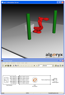
Fig. 51.4 Model view and AGX Remote Debugger view of example scene.
The view can be changed (rotated, zoomed, panned) using the mouse.
For a list of available key bindings of the agxViewer application, see Table 29: Keyboard bindings.
On some systems, you might get warnings from your firewall when using the remote debugger for visual output, since data is sent via a socket on localhost from the plugin to the general AGX application. No internet connection is needed, so refusing the application connection to the internet should not impede the functioning of the program. If your firewall settings do not allow the opening of a socket on localhost and you do not want to/cannot change that, you might have to fall back to using the plugin without the visual output via remote debugger (and thus without graphics).
51.6. Defining input and output signals
The coupling between Matlab/Simulink and AGX Dynamics is done by setting up callback functions. These functions will be called at initialization or every time step for reading input and output data. Below is an example written in Python.
This example scenario consists only of one rigid body, a box, which is rotating along a hinge which is fixed in the world coordinate system. It receives one input per time step: The speed of the hinge motor. The simulation has one output per time step: The summed-up angle of rotations around the hinge axis (this angle can thus be \(> 2 \pi\) or \(< -2 \pi\) in case of several full rotations).
The following two subsections will explain how this input and output values are defined in Python.
51.6.1. Python
Here we will use <AGX-dir>/data/matlab/scripts/rotatingBox.py as an example.
51.6.1.1. Defining the parameters
When loading the Python script, AGX will first parse it and execute all commandos which are not inside in a function, that is all code in global scope.
Note
Inputs and outputs (both for scene initialization and step-function) have to be defined outside of functions (global scope).
The scene itself is defined in the function buildScene() in the Python script. This function will load the simulation scenario.
In the simple case of the example file, the whole scene is setup directly in this Python function. In more complex cases, you might want to call one or several separate Python files to set up the scene, or load in data from other files.
The input signals (data from matlab to AGX) and output signals (data from AGX to matlab) are implemented in classes derived from the class agxMex.PythonControlArgument:
class HingeSpeedInputControl(agxMex.PythonControlArgument):
    def __init__(self, numInput, numOutput):
        # Call the constructor of PythonControlArgument
        # Specify the number of input and output variables
        super().__init__(numInput, numOutput)

    # This method is called at the startup of the simulation
    # It will get the intialization data from Matlab/simulink
    def input(self, sim, data):
        speed = data[0]
        constraint = sim.getHinge("Hinge")
        assert constraint
        motor = constraint.getMotor1D()
        motor.setSpeed(speed)
        return True

    # This method will be called every time step
    # Reading data from AGX and feeding it back to Matlab/Simulink
    def output(self, sim, data):
        assert(len(data) == 1)
        constraint = sim.getHinge("Hinge")
        assert constraint
        # read output data from simulation
        angle = constraint.getAngle()
        data[0] = angle
        return True
The init input control and the output control is then registered with the following lines:
# Specify number of input/output variables
numInput = 1
numOutput = 1
argA = HingeSpeedInputControl(numInput, numOutput)

# Register the Input port (to AGX) to the controller
agxSDK.SimulationControl.instance().addInitInputArgument("HingeSpeedInput", argA)

# Register the Output (from AGX) port to the controller
agxSDK.SimulationControl.instance().addOutputArgument("HingeAngleOutput", argA)
51.6.1.2. Evaluating inputs and outputs
Each time step, AGX does the following three steps:
Call all input functions in the order of their declaration in the Python script, making use of the input from Simulink to control the AGX simulation.
Take one simulation step.
Call all output functions in the order of their declaration in the Python script, writing results from the AGX Simulation back into the Simulink output data.
51.6.1.3. Initialization input and output
If you want to make the scene setup depend on parameters, you can set these using the function:
agxSDK.SimulationControl.instance().addInitInputArgument(<object derived from agxMex.PythonControlArgument>)
where <InputArgument> is the same kind of argument as for:
agxSDK.SimulationControl.instance().addInputArgument(<Object derived from agxMex.PythonControlArgument>)
If you want to get one-time output from the scene initialization, this can be specified using the function:
agxSDK.SimulationControl.instance().addInitOutputArgument(<object derived from agxMex.PythonControlArgument>)
- The order of execution at scene initialization is:
Parse Python script, and register all arguments which must be added to agxSDK.SimulationControl.
Execute all instances of agxMex.PythonControlArgument added with addInitInputArgument
Execute the function buildScene().
Execute all instances of agxMex.PythonControlArgument added with addInitOutputArgument
51.7. Examples
51.7.1. MatLab
Examples of matlab scripts which how to use the AGX-Matlab connection is located in <AGX-dir>\data\Matlab\
All corresponding Python scripts are located in <AGX-dir>\data\Matlabscripts
To run an example, start Matlab, change directory to <AGX-dir>\dataMatlab\ and enter the name of the matlab script.
51.7.2. Simulink
Examples of Simulink projects which demonstrates the AGX-Simulink connection is located in located in <AGX-dir>\dataMatlab\simulink\
51.8. Limitations
This version of the Matlab/Simulink integration has several limitations.
Dynamically linked libraries like agxMex.dll, agxCore.dll, agxPhysics.dll and agxOSG.dll will not be unloaded once they have been loaded in Matlab, until Matlab is shut down.
You cannot use Matlab and Simulink in the same session. Please restart Matlab if you are working with the Matlab connection and need to use Simulink.
Only one AGX block allowed per model.
After the Matlab command clear has been executed, AGX should not be used (this includes also calls to clear mex or clear all).