17. Plot Tool

The plot tool can be used for plotting live data during a simulation or from a recorded simulation. The plotting also allows for comparison plots between different recordings.
Note
The plotting is depending on the Recording Frequency
17.1. Units
All units in the plotting tool is in SI units:
Time - s
Distance - m
Linear speed - m/s
Angular speed - rad/s
Linear Acceleration - m/s^2
Angular Acceleration - rad/s^2
Force - N
Torque - Nm
17.2. Plot interface
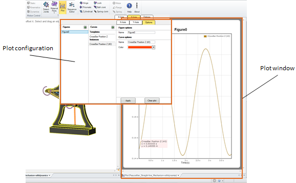
The plot consists of two windows: plot configuration and plot window. The plot can be setup and configured in the plot configuration. The plot window will contain the figures and curves that have been specified.
17.3. Plot configuration
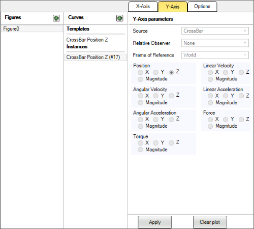
The plot configuration is available from the plot tool in the ribbon. It consists of three sections: Figures, Curves and Parameters.
17.3.1. Figures
A figure is a section in the plot window where curves are displayed as a sub-window of the Plot window. Adding a figure is done by pressing the ‘+’ button in the top left corner of the figures section. Deleting a figure is done by selecting it and pressing the delete button on the keyboard.

17.3.2. Curves
The curve section consists of two parts: Templates and Instances.

Templates are configured curves within a figure that will generate Instances of curves for every new simulation being recorded. So everytime a new simulation (new initial state) is being recorded, each template will result in a corresponding instance of a curve. This allows for comparison between different simulation configurations.
For example, you can setup your simulation, create a template for a curve, simulate. Investigate the result, then if you change your model by modifying geometry or any other Momentum property you can record a new simulation which will show up as a new instance of a curve for the same template. This allows for instant comparison.
You can delete an instance or template by selecting the curve and press the delete button. Instances are stored within the journal file. So even if the source of the data is removed, for example if you delete a joint for which there is a curve, the instance of the curve for that joint will still remain in the plot until you explicitly delete it.
17.3.2.1. Naming of curves
By default the name of a curve relates to the initially selected source of data and the selected component. So selecting Hinge 17 and selecting source motor torque will generate a curve template named Hinge 17 Motor Torque.
Instances will also be appended with a number (#2) indicating the n:th simulation of the model. Simulating a model (simulation #1), changing a physical property will result in an incremented simulation number (#2) etc.
You can at any time change the name of a curve template or an instance with the Options tab.
17.3.3. Options
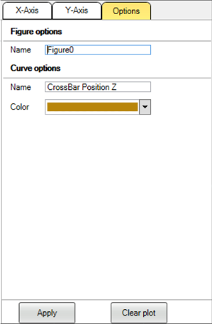
Figure options Name - Change the name of the current figure.
Curve options Name - Change name of the currently selected curve Color - select the color of the currently selected curve
The Apply button will commit the current changes into effect for the plot window. So changing the color of an instance of a curve will not be visible until the Apply button is pressed.
The Clear plot button is described below.
17.3.4. Parameters
17.3.4.1. Source
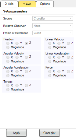
Here you select the source of data that you want to plot. By default the time is used as the value for the X-axis. The unit for time is always seconds (s). You can also change the source of data for any selected template of a curve. If a recorded simulation exists, a new instance of that curve will be created. By default, the name of the curve relates to the source of data.
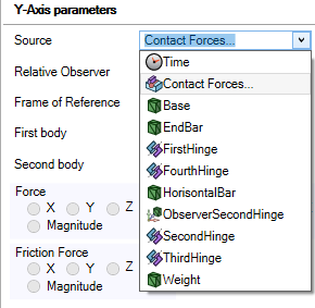
Fig. 17.1 Plot source drop down menu
The available sources for plotting are:
Joints
RigidBody
Observer
Contact forces
Time
Depending on which source of data that currently selected, there are different data points available:
Position
Linear velocity
Angular velocity
Linear Acceleration
Angular Acceleration
Force
Torque
Joint data
17.3.4.2. Plotting Contact forces
The contact forces (normal and friction force) can be plotted between two rigid bodies by choosing the Contact Forces ( ) item in the Source drop down menu.
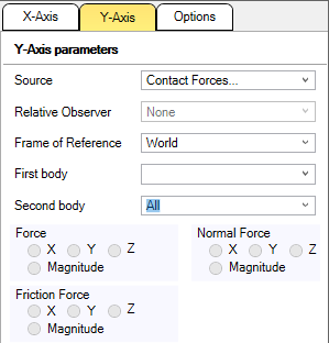
Fig. 17.2 Parameters for plotting Contact Forces
Frame of Reference - Specifies an observer in which coordinate system 3D data will be plotted. See Section 17.3.4.4
First body - Specifies the first rigid body which is involved in the contact data we want to plot.
Second body - Specifies the second rigid body which is involved in the contact data we want to plot. All indicates that contacts between the First body and all other bodies will be included in the data.
The available data for Contact Forces are:
Force - The total force applied as a contact (normal and friction) between the two rigid bodies
Normal Force - The force applied to avoid penetration between the two rigid bodies
Friction Force - The frictional force applied orthogonal to the normal force between two rigid bodies. To get accurate results, you might want to choose the Direct solver for the material pair of the two interacting rigid bodies.
Note
The plotting of contact data is filtered using a median filter of size 6. This means that the value reported is the average of the last 6 read values. If you want to access the raw data you can do this with the Python scripting API
17.3.4.3. Relative Observer
An Observer is a coordinate system which can either be fixed to the world or attached to a solid of a rigid body. If the rigid body moves, the observer will follow its movement, hence creating a moving coordinate system.
A relative observer can be used to plot the difference between two observers speed, acceleration or position. Consider the example in Fig. 17.3
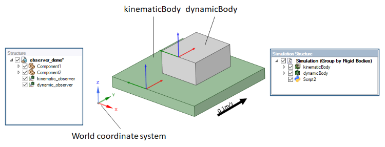
Fig. 17.3 Example with two Observers each attached to a rigid body.
The green box is a kinematic body with linear velocity in Y=0.1m/s. The gray box is a dynamic body standing on top of the kinematic body, hence they are moving together.
kinematic_observer is attached to the kinematic body. dynamic_observer is attached to the dynamic body.
If we want to know the difference in linear speed between the two Observers, we can:
Choose source: kinematic_observer
Choose Relative observer: dynamic_observer
Choose Linear Velocity/Magnitude
This will plot the relative velocity between the two observers in the world coordinate system. The same can be used for position and acceleration.
17.3.4.4. Frame of reference
By default all 3D data (position, velocity, acceleration, forces, torques) are plotted in the world coordinate system.
If you want to choose a different coordinate system in which you want to plot your data you can choose an Observer as a Frame of reference.
If an observer is attached to a moving rigid body, the coordinate system for that observer will also move. This can be useful if you for example want to measure the torque that a joint applies onto a body in a specific local orientation system to the body.
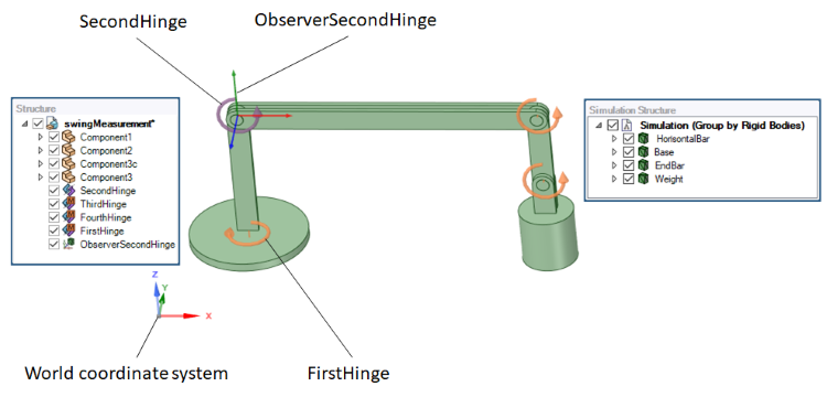
Fig. 17.4 Example of an Observer attached to a moving rigid body to create a local coordinate system.
In Fig. 17.4 we have a hinge (SecondHinge) attached between the vertical and the horisontal bar. If we want to investigate the torque being applied by the SecondHinge onto the first rigid body, we can choose the settings as seen in Fig. 17.5.
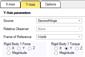
Fig. 17.5 Rigid Body 1 torque in Y-axis selected for SecondHinge.
This results in the plot Fig. 17.6
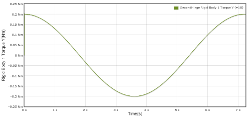
Fig. 17.6 Plotting Hinge torque in Y-axis for the world coordinate system.
However, if we instead want to see the torque in the local coordinate system of the SecondHinge, we can instead choose the ObserverSecondHinge as the Frame of reference:
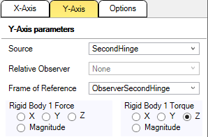
Fig. 17.7 Rigid Body 1 torque in Z-axis selected (the blue axis of the ObserverSecondHinge) for SecondHinge with ObserverSecondHinge as Frame of reference.
This results in the plot Fig. 17.8
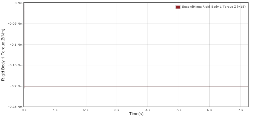
Fig. 17.8 Plotting Hinge torque in Y-axis for the local coordinate system of ObserverSecondHinge.
17.4. Plot window
The plot window contains all the figure and curves for the current document.
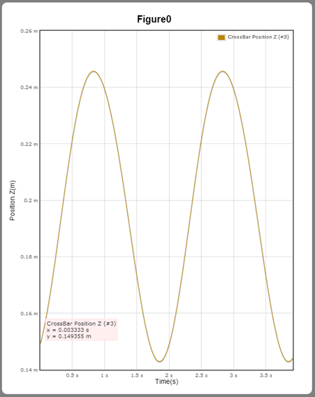
The window can be docked (or floating) as any other window in SpaceClaim. However, docking and position configuration will not be stored between sessions in SpaceClaim.
Moving the mouse in the window will show the current value for the curve closes to the mouse pointer.
Panning - Panning is done by a click and drag with the right mouse button, moving up/down left/right.
Zooming - Zooming is done by left-mouse box-selecting an area of interest or by using the mouse scroll.
17.5. Clear Plot
The Clear plot button will remove all plot instances. This quickly removes all data if it is outdated. If you want to just plot data from the current simulation, you can press Clear plot and then Apply.This will remove all stored plots and then recreate the current ones. There is one Clear Plot button in the Plot Options and one in the drop down menu of the ribbon.
17.6. Workflow
First open up the Plot configuration by pressing the plot button in the ribbon.
Click on a figure in the list of figures, or press the + button to create a new figure. Additional figures will be shown after each other in the plot window.
For the selected figure, press the ‘+’ button in the curve section to create a new curve.
Select the new curve and specify the desired data source for the X-axis and the Y-axis in the parameters section.
Name and color of the curve can be changed in the options tab.
17.7. Exporting data
Data can be exported from a plot figure with a right click with the mouse over the plot window.
