19. Script Editor¶

The Script Editor utilizes the Python scripting language together with the Momentum Scripting API to allow for writing scripts which are executed during the simulation or during playback of a previously recorded simulation.

A script can either read data from or write data to the current simulation. With a script you can write a controller which controls for example the motor speed based on data read from the simulation.

There are two types of scripts:

Script type	Write data	Read data	Discards recorded simulation
Simulation	Yes	Yes	Yes
Analysis	No	Yes	No

Attention

Because a Momentum script can access the local file system you should treat documents with scripts with care. You can disable all scripting in the current document with the Scripting Enabled button in the Playback Tab.

When opening a document containing scripts for the first time, this warning will be shown:

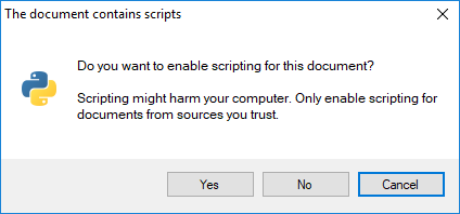
Answering Yes will enable scripting for the document. The next time a document with the same path will be opened, scripting will be automatically enabled. Answering No will disable the scripting for the document. You can enable the scripting feature later in the playback tab.

Note

Similar to plotting, the units being used through out the Momentum scripting are SI-units such as: meter, seconds, radians, Newton, Newton meter, etc.

19.1. Installing additional python packages¶

By default, an embedded Python environment is used in Algoryx Momentum. This means that the Python compiler as well as the standard libraries in use are pre-installed with Algoryx Momentum. If you want to use additional modules not available in the The Python Standard Library or numpy which comes with the installation, you can switch to your own Python installation. Read more about how to do this in the Python section of add-in options.

To install additional packages, follow the standard procedure for adding packages in Python using the ‘pip install’ command. When you have changed to your own Python installation using the addin-options in Algoryx Momentum (and restarted SpaceClaim) the new modules will be available in the script editor.

Attention

It is very important that you use the exact same version/library of Python that was used when building Algoryx Momentum. You can find 64-bit installers for Python here. Which version of Python that is currently used can be displayed using the About button in the Info section.

19.2. Simulation script¶

A Simulation script can read from and write data to the simulation. This allows for writing controllers that read data and calculate a response which is then written to the simulation. This workflow allows for controlling the speed on a motorized hinge or moving a kinematic rigid body according to data read from the simulation.

Note

Notice that changing the state in a script will NOT affect the initial state in any of the property settings for Momentum.

19.3. Analysis script¶

An Analysis script can only read data from the simulation. An analysis script can be attached to a simulation without discarding the current recording. This makes it suitable for reading data from an already existing recording.

Note

If you are executing an Analysis script on a pre-recorded simulation, you might discover that the script is not executed with the same frequency as when it was recorded. This is because simulations can be recorded in a frequency that is lower than that it is simulated. See Simulation Frequency vs. Recording Frequency.

19.4. Scripting API¶

The detailed documentation of the Python API for reading/writing data in a simulation can be read here: Momentum Script API Documentation

19.5. Script execution flow¶

Execution flow of a Momentum script show the execution process of a Momentum script. The user can write code for each of the functions: OnStart(), OnStep() and OnStop()

Fig. 19.1 Execution flow of a Momentum script¶

Note

OnStep() is called after a step in the Dynamic simulation. So for example, if you need to add a force for a rigid body, you might consider to call addForce for that body also in OnStart(). Otherwise no force will be added for the first time step.

On the other side, in OnStep() all forces (from joints and contacts) are available because the step in the Dynamic simulation is already done.

19.6. Breakdown of a script¶

A Momentum script has four parts:

The Global scope

from Momentum import v1
import math

# Access the simulation using:
sim = v1.getSimulation()

hinge = sim.getHingeJoint("motorHinge")
assert hinge

avgTorque = 0
sumTorque = 0
numSteps = 0

The OnStart function

def OnStart(time):
    hinge.getMotor().setEnabled(True)

The OnStep function

def OnStep(time):
    global numSteps
    global sumTorque
    hinge.getMotor().setTargetSpeed( 10*math.sin(time) )
    torque = hinge.getMotor().getCurrentTorque()
    numSteps +=1
    sumTorque += torque

The OnStop function

def OnStop(time):
    if (numSteps > 0):
        print("AvgTorque: {} Nm".format(sumTorque/numSteps) )
    else:
        print("No torque available")

Table 19.1 Execution of pre-defined functions¶
Function	Simulation Script	Analysis Script
Global scope	Executed when a new recording is started	Executed when a recording or playback is started
OnStart	Triggered at start of recording of a simulation	Triggered at start of recording and playback of a simulation
OnStep	Triggered at each step during recording of a simulation	Triggered at each step during recording and playback.
OnStop	Triggered at the end of a recording	Triggered at the end of recording and playback

Table 19.1 show when the pre-defined functions of a momentum script are executed.

19.6.1. The Global scope¶

This is usually where you import your required modules. Note that the internal python included in Algoryx Momentum only comes with the Python Standard Library plus numpy. A thorough list of available standard libraries for Python can be found at: The Python Standard Library

The Global scope can also be used to declare variables that are supposed to be available throughout the script. The code in the global scope is only executed when you press the Simulate button ( SIMULATION_SIMULATE ) or the Step button ( SIMULATION_STEP ).

Note

Changing the current time using the time slider or the step buttons in the Playback Tab will not execute the code in the global scope.

If you need additional modules, see how to change to an external interpretator at python options.

19.6.2. The OnStart function¶

This function is called at the start of a simulation recording or playback. This is a typical place for adding code that setup the initial state of the simulation or open files for writing. The current time of the simulation can be read in the argument time.

19.6.3. The OnStep function¶

This function is called at each time step during recording and at every recorded time step during playback. The current time of the simulation can be read in the argument time.

The reason why the number of calls to this function might differ between recording a simulation and playback of a simulation is due to the specified recording sampling rate.

This function is the heartbeat of your simulation. This is where you can add the code for reading and writing data.

Note

Printing text to the console might slow down the simulation considerably, especially at high simulation frequencies.

19.6.4. The OnStop function¶

This function is called when the recording or playback of a simulation is stopped. This can happen when:

When the user press the stop button ()
After the step button () is pressed
When the end of time is reached during both recording and playback

19.7. The script editor UI¶

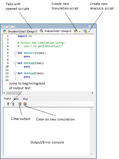
Fig. 19.2 The Python script editor.¶

The tabs () show the name of the script and the associated document within parenthesis.
The two buttons () at the right in the script editor tab is used to create either a Simulation script or an Analysis script.
The two buttons is used for jumping to the first/last line in the output/error window.
- Will clear the output/error window
When the Clear on new simulation button () is toggled, the output/error will be cleared at each new simulation.

19.8. Error¶

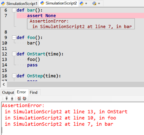
Fig. 19.3 Error shown in the script editor.¶

Whenever an error occurs in the executed script, it will be highlighted in the editor and written to the error console. The error message in the editor window will be in short form, whereas the error in the error console will contain the full traceback of the error call.

The script error will also be written to the Spaceclaim Status history at the bottom row in the Spaceclaim UI. Clicking an error message will take you to the script that contains the error.

Note

Errors in external scripts will not be highlighted in the Script editor. You need to edit external scripts with an external editor.

19.9. Find¶

The following keyboard shortcuts will open a find widget:

Key	Description
Ctrl+f	Find text
Ctrl+h	Find and replace text
Ctrl+g	Goto specified line
F3	Find next
Shift+F3	Find previous

19.10. External script and modules¶

Additional python modules and script files on your computer can be accessed by adding a path to the Python Environment Path. Another option is to do this from within the script:

import sys
externalPath = 'c:\\myScripts\\'

if (not externalPath in sys.path):
  sys.path.append(externalPath)

Notice the use of ‘\\\\’ in the path. If you are unsure how the path are formatted you can call `print(sys.path)` to see the list of search paths.

Python will by default cache the compiled scripts after it has once been imported. Assume you have added a path to a directory containing a script named `myPythonScript.py`, you can than import that script into your Momentum script:

import importlib

import myPythonScript
importlib.reload(myPythonScript)

# Now call a function in the myScript module:
myPythonScript.myScriptFunction()

Note

Analysis scripts and Simulation scripts differs in when the global context and consequently the import is performed, see Table Execution of pre-defined functions.

19.11. Drag-drop scriptable objects¶

To exemplify how to access objects in the scripting API, it is also possible to drag and drop objects into the scripting editor. This will create a code snippet that return a reference to the specified object.

Fig. 19.4 Result of drag dropping a Hinge into the script editor.¶

Objects that can be drag dropped are:

RigidBodies
Joints
Observers

Note

If you change the name of an object after you have dropped the object into the editor, you will no longer get a correct reference.

19.12. Example scripts¶

Below are a few example scripts that show how to access objects in a Momentum script:

19.12.1. Using observers¶

If a simulation contains an Observer it can be accessed via it´s name by a call to the method getObserver:

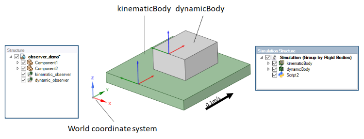
Fig. 19.5 Example with two Observers each attached to a rigid body.¶

sim = v1.getSimulation()
observer = sim.getObserver("dynamic_observer")

def OnStep(time):
  # Get the velocity of the dynamic_observer attached to the gray dynamic rigid body
  world_velocity = observer.getVelocity()
  print("World Velocity: ", world_velocity)

  # Use the observer to transform the velocity to its local coordinate system:
  local_velocity = observer.transformVectorToLocal(world_velocity)
  print("Local Velocity: ", local_velocity)

The output from this script would then be:

World Velocity:  [ -3.96713e-19, 0.1, -7.16121e-16]
Local Velocity:  [ 0.1, 5.89389e-08, -7.15339e-16]

The velocity of the dynamic_observer is 0.1 in Y in the world coordinate system. However, in the local coordinate system it is 0.1 in X.

19.12.2. Accessing Joints¶

There are several ways you can access Joints in Momentum scripting. By name:

sim = v1.getSimulation()
hinge = sim.getJoint("Hinge1")

The above code will give you a reference to the Joint. However, the type will be Joint, so you can only access methods available in the Base class Joint. If you want to use it as a HingeJoint, you can write:

sim = v1.getSimulation()
hinge = sim.getJoint("Hinge1")

# Cast the Joint to a HingeJoint to access the API for the class HingeJoint
hinge = hinge.asHingeJoint()

# Disable the motor for the HingeJoint:
hinge.getMotor().setEnabled(False)

You can also find the HingeJoint in the simulation by name:

sim = v1.getSimulation()
hinge = sim.getHingeJoint("Hinge1")
# Now you can use it as a HingeJoint directly
hinge.getMotor().setEnabled(False)

If you want to operate on many Joints at once, you can get a list of all joints:

sim = v1.getSimulation()
# Get all joints in the system
joints = sim.getJoints()

# Loop over all joints, if it is a Hinge, disable the motor
for j in joints:
  hinge = j.asHinge()
  if hinge:
    hinge.getMotor().setEnabled(False)

sim = v1.getSimulation()
# Get all joints in the system
joints = sim.getHingeJoints()

# Loop over all HingeJoints and disable motor
for j in joints:
  j.getMotor().setEnabled(False)

19.12.3. Applying Torque to a RigidBody¶

Rigid bodies can also be accessed by name or in a list just like joints. The code snipped below will add a constant torque to a rigid body (applyTorque()) Another function will calculate a breaking force depending on the angular velocity (brake()). The result can be seen in Fig. 19.6 is a simulation where the angular velocity of the rotating shaft reaches some oscillating state.

sim = v1.getSimulation()
body = sim.getRigidBody("inputShaft")

def brake():
  speed = body.getAngularVelocity().length()
  # Apply a breaking torque due to rotational speed
  body.addLocalTorque(0,0,-1*speed*speed)

def applyTorque():
  # Apply 10Nm around the local z-axis of the rigid body
  body.addLocalTorque(0,0,10)

# We apply the torque both in OnStart() and in OnStep()
def OnStart(time):
  applyTorque()
  brake()

def OnStep(time):
  applyTorque()
  brake()

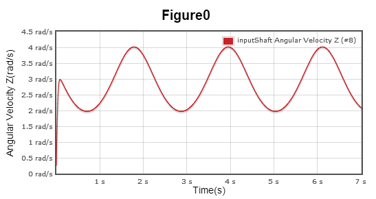
../_images/ScriptEditor_addTorquePlot.png

Fig. 19.6 Angular velocity for the rotating shaft¶

19.12.4. Accessing Motor, Range and Spring¶

Some joints such as HingeJoint, PrismaticJoint, and CylindricalJoint have some additional SecondaryJoints. See for example Motor.

These SecondaryJoints can be accessed in the Momentum scripting API to control speed, range, torque and force limits.

sim = v1.getSimulation()
hinge = sim.getHingeJoint("Hinge1")
assert hinge

# We set some initial state for the motor:
def OnStart(time):
    # We specify the amount of torque available in negative/positive direction
    hinge.getMotor().setTorqueLimit((-5,5))

    # We make sure the motor is enabled
    hinge.getMotor().setEnabled(True)

    # We set a target speed for the motor
    hinge.getMotor().setTargetSpeed(1)

# Every time step we print the amount of torque applied by the motor
def OnStep(time):
    print("CurrentTorque", hinge.getMotor().getCurrentTorque())
    pass

19.12.5. Accessing contact data¶

There are several ways to access contact data depending on what is needed. Contact data is only available in the `OnStep()` function.

19.12.5.1. Accessing all contacts¶

To iterate over all available contacts, you can use the method `Simulation.getContacts()` without arguments:

def OnStep(time):
    contacts = sim.getContacts()
    for c in contacts:
        b1 = c.getBody1().getName()
        b2 = c.getBody2().getName()
        nf = c.getNormalForce()
        ff = c.getFrictionalForce()
        print("Body {0} <-> {1} => NormalForce: {2}, FrictionForce: {3}".format(b1,b2,nf,ff))

The code above could result in the following output for each simulation step:

` Body Component2 <-> Component1 => NormalForce: [ -0, -0, 0.589931], FrictionForce: [ -0, -0, 0.589931] `

19.12.5.2. Accessing contacts for specific bodies¶

The method `Simulation.getContacts()` can also have one or more arguments which narrows down the selection of contacts.

To get a list of all contacts for a specific rigid body:

def OnStep(time):
    body = sim.getRigidBody("myBody")
    assert body # Make sure we did find a body named "myBody"
    # Get contacts where the body "myBody" is involved.
    contacts = sim.getContacts(body)

Note

The python type None is used as a wildcard for matching objects in the call to `Simulation.getContacts()` This means that if you call to for example `sim.getRigidBody("myBody")` fails and returns None, it will match any rigid body. So make sure that your argument are not None using for example assert.

19.12.5.3. Accessing accumulated contact forces¶

There are several methods available for accessing accumulated contact forces acting upon a rigid body.

def OnStep(time):
    body = sim.getRigidBody("myBody")
    assert body # Make sure we did find a body named "myBody"
    # Get the sum of all normal forces acting upon the body:
    accNormalForce = sim.getNormalContactForces(body)

19.12.5.4. Filtering contact data¶

The plotting of contact forces is utilizing a filter for the display of contact data. If you want to the same filter when accessing data through the script API you can do this by utilizing the class `MedianStatistic`.

First you need to create an instance of the filter for each data point that you need to filter, for example magnitude of the normal contact force:

# Create a filter with the number of observations set to 6
normal_contact_force_magnitude_filter = v1.MedianStatistic(6)

def OnStep(time):
    # Get contact data as in the previous example:
    body = sim.getRigidBody("myBody")
    assert body # Make sure we did find a body named "myBody"

    # Get the sum of all normal forces acting upon the body:
    accNormalForce = sim.getNormalContactForces(body).length()

    # Feed the raw data into the filter:
    normal_contact_force_magnitude_filter.update( accNormalForce )

    # Now get the smoothed value
    filtered_value = normal_contact_force_magnitude_filter.get()

19.12.6. Controlling gravity¶

Below is a short example of changing the the gravity during a simulation:

from Momentum import v1
import math

sim = v1.getSimulation()

def OnStep(time):
    # Default gravity vector as set in Simulation settings
    g = sim.getGravity()

    # Calculate a rotation in radians
    y = math.sin(time)*math.pi

    # Apply the rotation around Y
    e = v1.EulerAngles(0,y,0)
    # Create a rotation matrix
    m = v1.AffineMatrix4x4()
    m.setRotate(e)

    # Calculate a new gravity vector by rotating the original vector
    g_new = m * g

    # Apply the new gravity
    sim.setGravity(g_new)
    print(g_new)
    pass

def OnStop(time):
    pass

19.12.7. Granular¶

Note

Feature requires a Momentum Granular license.

Most of the granular objects in the scene can be accesed and controlled via the API, such as Emitters, Sensors, granular bodies and granular contacts.

19.12.7.1. Creating Granular Bodies¶

Below follows a short example script for creating a column of granular bodies and extracting information about them.

from Momentum import v1
import random as rand

sim = v1.getSimulation()

def OnStart(time):
if time == 0:
  # Extract the granular body system in the simulation
  granularBodySystem = sim.getGranularBodySystem()
  mat = sim.getMaterial("Granular")
  # Granular Bodies are created via the GranularBodySystem object extracted from the simulation
  # Create a column of 10 particles with radomized radius
  radius = 0.01
  increment = radius * 2
  for i in range(0,10):
      # Randomize a new radius given an increment interval
      newRadius = radius + rand.random() * increment
      # Create a new particle with the new radius and extract material
      granularBody  = granularBodySystem.createGranularBody(newRadius, mat);
      # Generate and set new position
      position  = v1.Vec3(0,0, 2 * radius + i * (2 * radius + increment))
      granularBody.setPosition(position)
      # Set random particle color
      granularBody.setColor(v1.Vec4(rand.random(), rand.random(), rand.random(), 1.0))

def OnStep(time):
  # Get GranularBodySystem from the simulation
  granularBodySystem = sim.getGranularBodySystem()

  # Extract bodies from the GranularBodySystem container
  granularBodies = granularBodySystem.getGranularBodies()
  for b in granularBodies:
    print(str(b.getId()) + " : " + str(b.getPosition()))
  pass

def OnStop(time):
  pass

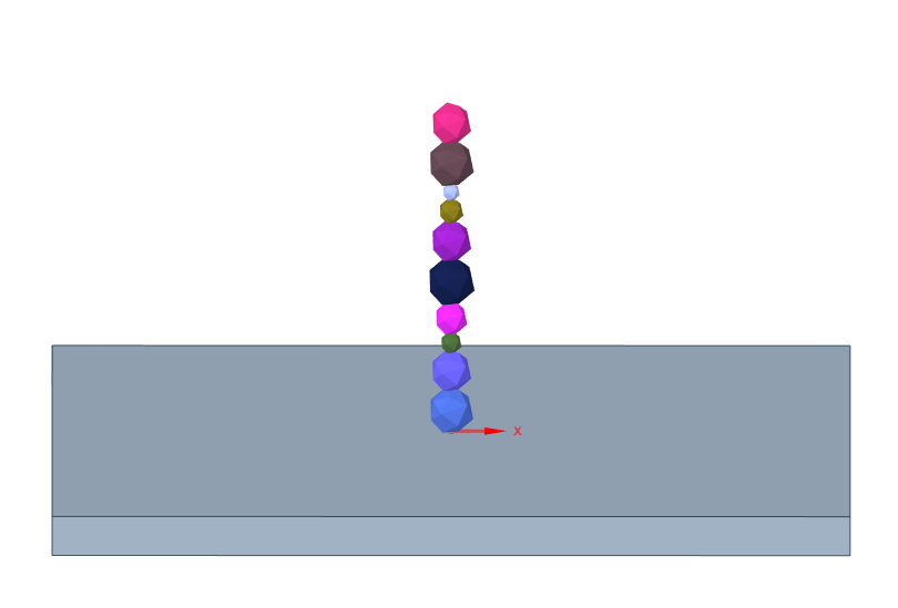
Fig. 19.7 Vertical Granular column with particles of different properties created via Python scripting.¶

19.12.7.2. Creating Granular Body Lattices¶

Below follows an example script for creating a lattice structures of Granular Bodies. These structures can be created either by specifying bounds in the scene or by creating them in a geometry active in the scene. The lattices can be constructed in different formats depending on the use case.

Lattice Type	Description
SQUARE_PACK	Will create a Granular Body lattice in a square pattern.
HEXAGONAL_CLOSE_PACK	Will create a Granular Body lattice in a close-packed hexagonal pattern.

from Momentum import v1
import math
import random as rand

# Access the simulation using:
sim = v1.getSimulation()

def OnStart(time):
  if time == 0:
    # Create Particles
    gsystem = sim.getGranularBodySystem()
    material = sim.getMaterial("Granular")

    # Setup dimensions of the lattice
    radius = 0.1
    startPos  = v1.Vec3(5,0,0)
    minVec    = v1.Vec3(-1.5,-1,3)
    maxVec    = v1.Vec3(1.5,1,7)

    # First, create a lattice with the default configuration of a SQUARE_LATTICE
    max = maxVec - startPos
    min = minVec - startPos
    granulars = gsystem.spawnGranularBodyLatticeInBound(min, max, radius, v1.Vec3(2*radius,2*radius,2*radius), 0, material, v1.GranularBodySystem.SQUARE_PACK)

    # Second, create a lattice with the configuration of a HEXAGONAL_CLOSE_PACK
    max = maxVec + startPos
    min = minVec + startPos
    granulars = gsystem.spawnGranularBodyLatticeInBound(min, max, radius, v1.Vec3(2*radius,2*radius,2*radius), 0, material, v1.GranularBodySystem.HEXAGONAL_CLOSE_PACK)

    # Thirdly, create a lattice with the configuration of a HEXAGONAL_CLOSE_PACK inside a solid inside the simulation
    spawnGeom = sim.getGeometry("SpawnGeom")
    granulars = gsystem.spawnGranularBodyLatticeInGeometry(spawnGeom, radius, v1.Vec3(2*radius,2*radius,2*radius), 0, material, v1.GranularBodySystem.HEXAGONAL_CLOSE_PACK)
    # Modify the granulars created by the previous lattice creation
    for b in granulars:
        r = radius - (rand.random() * (0.2*radius))
        b.setRadius(r)
        b.setColor(v1.Vec4(.3, .3, .3, 1.0))
        b.setRotation(v1.EulerAngles(rand.random()*2.0*math.pi, rand.random()*2.0*math.pi, rand.random()*2.0*math.pi))

def OnStep(time):
    pass

def OnStop(time):
    pass

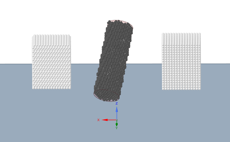
Fig. 19.8 Figure of different lattice constructions of Granular Bodies: Hexgonal-Close-Pack (left), Hexgonal-Close-Pack inside a solid (middle) and a Square Lattice Pattern (right).¶

19.12.7.3. Writing and Reading Granular States¶

There are methods for writing and reading granular body data to external files, similar to the snapshot functionality in Sensors. This functionliy will store the granular data to the AGX Dynamics .agx format, which can be loaded into other environments that use AGX Dynamics. In order to write the current granular state to disk, use the following code snippet:

# This function call will store all granular bodies in the scene to an .agx file.
success = granular_system.writeFile( "stored_granular_bodies.agx",
                                     granular_system.getGranularBodies() )

You can also limit the granulars stored to those that are inside a geometric bound in a simulation:

# Get the geometry that will serve as a bound for storing granulars
store_bound = sim.getGeometry("granular_store_bound")
success = granular_system.writeFileFromGeometry("stored_granular_bodies.agx",
                                                granular_system.getGranularBodies(),
                                                store_bound )

You can load granular snapshot files generated from script or from the new sensor snapshot functionality introduced in 2.3.0. An initial Material needs to be applied to the granular bodies when loading. This will determine the final mass of the granular bodies and also affect the contact interaction properties configured in Material Pairs. Two loading functions exists where one function returns the bodies loaded from the specified file while the other does not.

# Specify a material that will be applied to the granulars when loading.
initMaterial = sim.getMaterial("granular_material")
# You can give the loading function a vector where the granularBodies
# loaded granular bodies will be stored.
granularBodies = v1.GranularBodyVector()
# OPTIONAL - You can supply an optional transform argument that will be applied to
# granular position and velocity before storage.
transform = v1.AffineMatrix4x4()
success =  granular_system.loadFileGetBodies("stored_granular_bodies.agx",
                                             initMaterial,
                                             granularBodies,
                                             transform )

# The second function does not use the optional transform and granular body vector
success =  granular_system.loadFile("stored_granular_bodies.agx",
                                    initMaterial )

19.12.7.4. Accessing Emitted Rigid Body Data¶

Data about emitted Rigid Bodies are extracted from the v1::Simulation in contrast to granular body data which is accesed via the v1::GranularBodySystem object:

# Extract all rigid bodies that have been emitted
emittedBodies = sim.getEmittedBodies()

for body in emittedBodies:
  #... do v1::RigidBody operations ...
  pass

  # You can also check if a RigidBody is an emitted or loaded
  # NSS body by querying the "isEmittedBody" function
  for b in sim.getRigidBodies():
    isEmittedBody = b.isEmittedBody()

Emitted bodies are v1::RigidBody instances and can be manipulated as such.

There is also methods for writing both granular body and granular body:

# Extract all NSS bodies that have been emitted
emittedBodies = sim.getEmittedBodies()

# Extract all NSS bodies with the midpoint inside a specific geometry
filteredBodies = sim.filterRigidBodiesInGeometry(geometry,
                                                 emittedBodies,
                                                 True)

# Extract all granular bodies with the midpoint inside a specific geometry
granular_bodies = granular_system.filterBodiesInGeometry(geometry,
                                                         granular_system.getGranularBodies(),
                                                         True)

# This function call will store all NSS and granular bodies in the scene to an .agx file.
success = simulation.writeGranularFile("stored_bodies.agx",
                                       granular_bodies,
                                       emitted_bodies)

19.12.7.5. Emitters¶

Emitters can be extracted out of the simulation and controlled. Below follows a short example script for changning emitter rate over time.

from Momentum import v1
import math
import random as rand

# Access the simulation using:
sim = v1.getSimulation()

def OnStart(time):
    pass

def OnStep(time):
    # Extract emitter from the simulation
    emitter = sim.getEmitter("Emitter0")

    # Change emitter rate depeding on time
    rate = 100 * math.pow(math.fabs(math.sin(math.pi * time)), 2)
    print(str(rate))
    emitter.setMassFlowRate(rate)

    # Extract information about emitted quantities
    emittedMass        = emitter.getEmittedMass()       # Emitted mass in kg
    numEmitted         = emitter.getNumEmittedBodies()  # Number of emitted bodies
    maximumEmittedMass = emitter.getMaximumAllowedEmittedMass()  # Maximum emitted bodies
    pass

def OnStop(time):
    pass

19.12.7.6. Particle and Rigid Body Distributions¶

The user can also extract distribution data from emitters and used them to manually create objects from them:

GranularEmitter = sim.getEmitter("GranularEmitter")

# Make sure this is a "Particle" Emitter
assert GranularEmitter.EmitMode == v1.Emitter.PARTICLES
pdist = GranularEmitter.getParticleDistribution()
model = pdist.getRandomModel()
granularBodySystem = sim.getGranularBodySystem()

# Create a new particle instance from the model data
particle = granularBodySystem.createParticle(model.getRadius(), model.getMaterial())

RigidBodyEmitter = sim.getEmitter("RigidBodyEmitter")
# Make sure this is a "Particle" Emitter
assert GranularEmitter.EmitMode == v1.Emitter.RIGID_BODIES
nssdist = GranularEmitter.getBodyDistribution()
model = nssdist.getRandomModel()

# Create a new NSS rigid body instance from the model data
body = sim.createRigidBodyFromBodyModel(model, position, rotation, velocity)

19.12.7.7. Granular Contacts¶

There are several ways to access contact data between Granular Bodies themselves or between them and the objects in the simulation. The contact structure between Granular Bodies and Granular Bodies - Rigid Bodies are different since one of the contacts contain a rigid body instead of another Granular Body. Thus, we have two stypes of contacts that can be extracted from the simulation.

Contact Type	Description
Granular-Granular	Contact struct containing information about a Granular - Granular contact.
Granular-RigidBody	Contact struct containing information about a Granular - RigidBody contact.

Note

Accessing Rigid Body contact data is done in a similar way as with regular RigidBodies.

19.12.7.8. Accessing all granular contacts¶

To iterate over all available Granular-Granular contacts, you can use the method Simulation.getGranularContacts() without arguments:

def OnStep(time):
    contacts = sim.getGranularGranularContacts()
    for c in contacts:
        b1 = c.getGranularBody1().getId()
        b2 = c.getGranularBody2().getId()
        nf = c.getNormalForce()
        ff = c.getFrictionalForce()
        print("GranularBody {0} <-> {1} => NormalForce: {2}, FrictionForce: {3}".format(b1,b2,nf,ff))

The code above could result in the following output for each simulation step:

GranularBody 0 <-> 1 => NormalForce: [ -0, -0, 0.589931], FrictionForce: [ -0, -0, 0.589931]

To iterate over all available Granular-RigidBody contacts, you can use the method Simulation.getGranularRigidBodyContacts() without arguments:

def OnStep(time):
    contacts = sim.getGranularRigidBodyContacts()
    for c in contacts:
        b1 = c.getGranularBody().getId()
        b2 = c.getRigidBody().getName()
        nf = c.getNormalForce()
        ff = c.getFrictionalForce()
        print("GranularBody {0} <-> RigidBody {1} => NormalForce: {2}, FrictionForce: {3}".format(b1,b2,nf,ff))

The code above could result in the following output for each simulation step:

GranularBody 0 <-> RigidBody RigidBody2 => NormalForce: [ -0, -0, 0.589931], FrictionForce: [ -0, -0, 0.589931]

19.12.7.9. Accessing granular contacts for specific bodies¶

The method Simulation.getGranularRigidBodyContacts() can also have one or more arguments which narrows down the selection of contacts.

To get a list of all granular contacts for a specific rigid body:

def OnStep(time):
    body = sim.getRigidBody("myBody")
    assert body # Make sure we did find a body named "myBody"
    # Get contacts where the body "myBody" is involved.
    contacts = sim.getGranularRigidBodyContacts(body)

This also work for GranularBodies, except that the function Simulation.getGranularContacts(myGranularBody) is used instead.

Note

The python type None is used as a wildcard for matching objects in the call to Simulation.getGranularRigidBodyContacts() This means that if you call to for example sim.getRigidBody("myBody") fails and returns None, it will match any rigid body. So make sure that your argument are not None using for example assert.

19.12.7.10. Accessing accumulated granular contact forces¶

There are several methods available for accessing accumulated contact forces acting upon a rigid body.

def OnStep(time):
    body = sim.getRigidBody("myBody")
    assert body # Make sure we did find a body named "myBody"
    # Get the sum of all normal forces acting upon the body:
    accNormalForce = sim.getGranularRigidBodyNormalContactForces(body)

19.13. Limitations¶

When disabling a joint in joint properties the collision between the two bodies involved in the joint will be automatically enabled. However disabling a joint in a Simulation script with joint.setEnabled(False) will not enable the collision between the two bodies.

When using the Granular functionality inside a script environment, the granular plugin must be activated in order for a granular system to be added to the simulation.